

Abstract
The interdisciplinary nature of conservation problems is increasingly being incorporated into research, raising fundamental questions about the relative importance of the different types of knowledge and data. Although there has been extensive research on the development of methods and tools for conservation planning, especially spatial planning, comparatively little is known about the relative importance of ecological versus non-ecological data for prioritization, or the likely return on investment of incorporating better data. We demonstrate a simple approach for (1) quantifying the sensitivity of spatial planning results to different ecological and non-ecological data layers, and (2) estimating the potential gains in efficiency from incorporating additional data. Our case study involves spatial planning for coastal squeeze, a process by which development blocks coastal ecosystems from moving landward in response to sea-level rise. We show that incorporating spatial data on landowners' likelihood of selling had little effect on identifying relative priorities but drastically changed the outlook for whether conservation goals could be achieved. Better data on the costs of conservation actions had the greatest potential to improve the efficiency of spatial planning, in some cases generating more than an order of magnitude greater cost savings compared to ecological data. Our framework could be applied to other systems to guide the development of spatial planning and to identify general rules of thumb for the importance of alternative data sources for conservation problems in different socio-ecological contexts.
Export citation and abstract BibTeX RIS
Introduction
Conservation science is increasingly interdisciplinary, which introduces challenges associated with integrating knowledge and data from across a wide range of disciplines. Given ubiquitous limits on time and monetary resources, identifying which types of knowledge or data are most important for analyses meant to support conservation has wide relevance. This question is likely to be foundational for determining investment in data collection, forming interdisciplinary teams, and developing graduate education programs, among other activities in conservation science and education.
Much of conservation science and practice uses systematic planning, a framework for making the best use of the limited resources available for conservation (Margules and Pressey 2000, McCarthy et al 2012). Approaches to spatial systematic planning, in particular, are well established and the tools for implementing them are becoming increasingly sophisticated (e.g. Marxan; Watts et al 2009), but less is known about which types of knowledge or data are most important for ensuring that these tools lead to cost-effective decision-making. Ecological data are the foundation of most spatial planning because they are often necessary for measuring progress toward conservation goals and more familiar to conservation planners than social or economic data (Cowling 2014). Accordingly, much of the research on better understanding the sensitivity of spatial planning to the underlying data, and potential trade-offs associated with obtaining better data, is focused on different types of ecological data (e.g. Brooks et al 2004, Rondinini et al 2006, Grantham et al 2008).
Non-ecological data, and in particular economic costs and other social data, such as willingness to participate in conservation, can be an important component of efficient planning (e.g. Zhu et al 2015). It is not yet common practice, however, to incorporate a wide range of non-ecological data sources into planning efforts (Naidoo et al 2006, Naidoo and Ricketts 2006, Guerrero et al 2010, Knight et al 2010, Kujala et al 2018). One potential cause of this lag is that allocating greater effort toward non-ecological data sources is associated with trade-offs, including the potential to shift focus away from the biology of conservation (Arponen et al 2010), the cost of data collection, delaying action while waiting for better data (Grantham et al 2009), and the expertise needed to obtain and interpret additional data types. Incorporating multiple types of data, each of which has its own uncertainty, can also generate greater uncertainty in the results of the planning process. The potential costs of increased uncertainty include the need for more sophisticated, and potentially less accessible, planning tools that are capable of incorporating uncertainty, and less interpretable results, especially for non-specialist stakeholders.
There is currently little general guidance for navigating the costs and benefits of incorporating different types of data into conservation planning (Kujala et al 2018). To address this need, we first specify a framework for generating evidence that can be used to infer the relative importance of different data sources and quantify the influence of data layer accuracy, resolution and uncertainty. Our approach synthesizes a range of related approaches from planning research into three components designed to help planners navigate the trade-offs associated with choosing appropriate data types: (1) quantifying the sensitivity of conservation planning results to the types of data that are incorporated, (2) quantifying how much uncertainty is added from each data layer to visualize often overlooked trade-offs between greater uncertainty and greater efficiency, and (3) estimating the efficiency gains produced by each planning solution.
We used our approach to address two common spatial planning goals: estimating and ranking the conservation value of planning units and identifying a minimum set of planning units to meet conservation goals for the least cost. We determined the relative importance of the data types needed for these goals by quantifying the consequences of using coarser data layers that required less effort to obtain but are more typical of data used in spatial planning. We integrated three types of data—ecological, monetary cost, and human behavior—using complex datasets that do not typically exist for conservation planning in real-world contexts. For each of these three types, we compared the results obtained using these richer datasets to results obtained using more widely used data, including remote sensing of habitat layers, rapid count surveys, and county-level cost data. Previous studies have quantified the sensitivity of planning results to ecological and socio-economic data, either using widely available sources (Bode et al 2008, Carwardine et al 2010) or simulations (Kujala et al 2018), quantified the importance of human behavior data (Knight et al 2010), or characterized the uncertainty associated with integrating social data (Lechner et al 2014). Here, we use the richness of data for our system to extend these approaches by quantifying how sensitivity, uncertainty, and efficiency are influenced by relative investments into cost, human behavior, and ecological data, which have rarely been examined simultaneously.
We illustrate our framework using a conservation planning problem for a system that has a wealth of ecological data: the protection of tidal marshes and an endemic tidal marsh bird in Long Island Sound (LIS), USA. Approximately 5% of the US human population lives within 80 km of LIS, and the tidal marshes in this region lie within the core of the range of an endangered species, the saltmarsh sparrow (Ammospiza caudacutus, Wiest et al 2016). A primary conservation strategy for addressing coastal squeeze in this region, and the one considered here, is to protect sufficient land to allow marshes to migrate landward and mitigate losses from sea-level rise.
Methods
Data sources, conservation planning approach, and planning units
Our spatial planning objective was to identify planning units for the least cost that could provide (1) migration corridors for marshes and (2) the greatest protection to current saltmarsh sparrow nesting habitat. We defined costs according to the conservation action that is the focus of our planning (see Carwardine et al 2008), which is the cost of purchasing land in the coastal zone. We measured conservation value in relation to two targets: the projected extent of tidal marsh in 2100 assuming no additional barriers to marsh migration are constructed (Hoover 2009), and the current extent of saltmarsh sparrow nesting occurrence (Meiman and Elphick 2012). We also considered two lesser effort data sources that are potential proxies for saltmarsh sparrow nesting: saltmarsh sparrow abundance, estimated from count surveys (Wiest et al 2016), and the current extent of tidal marsh, estimated from remote sensing (Hoover 2009). We considered three goals that span the minimum and maximum extent likely to be set by practitioners: 33%, 66%, and 95% of each target's extent (or population when using abundance estimates as a proxy for nesting extent), allowing us to quantify the influence on our results of setting conservative versus ambitious goals.
We estimated the costs of properties within the migration zone using a Bayesian regression analysis of randomly selected properties from town assessors' databases (see SI is available online at stacks.iop.org/ERL/14/124081/mmedia). Unlike many proxies for costs, our statistical analysis of cost data resulted in a layer that meets important criteria for informing conservation planning as it captures the appropriate spatial variation (Armsworth 2014), which might not covary with conservation targets (Murdoch et al 2007). We compared this layer to a freely available, but less precise, proxy for land costs: county-scale, median values for agricultural land (US Department of Agriculture 2012). This cost proxy has been used to develop cost estimates for large-scale planning based on return on investment for the USA (Withey et al 2012). We estimated the proportion of landowners in each town who would be likely to sell their properties to a conservation organization for fair market value using data on behavioral intentions from a survey of >3000 landowners in the migration zone (Field et al 2017a). We quantified spatial variation in the proportion of landowners who would be likely to sell using a Bayesian logistic regression model with spatial random effects by town. We multiplied the proportion of landowners in each town who would be likely to sell their land by the extent of the migration zone to estimate how much of the migration zone is likely available for purchase, propagating confidence bounds of the estimation uncertainty of the statistical model (see SI for details on the statistical model and uncertainty propagation).
We defined planning units as cells (approximately 23 km2) in the hexagonal grid from the US Environmental Protection Agency's Environmental Monitoring and Assessment Program (https://archive.epa.gov/emap/archive-emap/web/html/). The planning units in this grid are large enough to encompass the larger marsh complexes in our study area and have previously been used to design sampling for estimating the abundance of saltmarsh sparrows (Wiest et al 2016). For each planning unit, we used the data listed above to calculate the 'fraction-of-the-spares' index (FOS), which estimates conservation value for prioritization or identifying a minimum set of planning units that meets goals for a set of conservation targets (Phillips et al 2010). The index uses data on the amount of each target in each planning unit to assign it a value between zero and one, with a value of one indicating that the planning unit is necessary for meeting conservation goals. We used the FOS because it estimates conservation value in relation to multiple targets, performs well compared to other conservation indices, and is straightforward to calculate and recalculate as necessary, facilitating the propagation of uncertainty of the underlying data layers. Because of its simplicity and intuitive scale, the FOS can also be easily communicated to a wide range of stakeholders. We divided the FOS index by the cost of land to obtain a benefit/cost ratio (Phillips et al 2010), which we used as our measure of conservation value. This general measure of return on investment, in which the 'investment' is the amount of the conservation target being protected, is an intuitive approach to planning that encourages efficiency (Murdoch et al 2007). We recalculated the FOS index for each planning unit 10 000 times, each time using independent draws from the uncertainty distributions for each data layer. The resulting confidence bounds represent the entire range of uncertainty contributed by the data layers that were used to calculate the index.
Sensitivity
Our 'best scenario' incorporated the best available data: projections of marsh migration, modeled saltmarsh sparrow nesting occurrence, land cost data from within the migration zone, and spatial data on likelihood of selling (table 1). We estimated conservation value for each planning unit for five alternative scenarios in which we either excluded a data layer (likelihood of selling) or replaced it with a reduced effort proxy (land cost, nest occurrence; see figure 1 for the scenarios). For each reduced effort scenario, we compared the conservation value of planning units to that obtained using the best scenario to quantify how sensitive these values were to the excluded data layer. First, we compared reduced effort scenarios to the best scenario using Spearman's rank correlations to estimate the similarity of the rankings produced by the FOS. We then calculated the number of planning units shared by each reduced effort scenario and the best scenario using a 10-planning unit moving window across the ranking from lowest to highest conservation priorities. This analysis gave a measure of similarity across the entire ranking and made it possible to determine whether, for example, there was high agreement between scenarios for the highest ranked planning units, but low agreement for the lowest ranked planning units. For example, a previous sensitivity analysis of cost data found low sensitivity to uncertainty for the highest and lowest ranked planning units (Carwardine et al 2010). We propagated the uncertainty of the FOS index for both analyses by calculating correlations for each of 10 000 independent draws of the index's uncertainty distribution. Together, these analyses quantify how successfully the reduced effort scenarios can approximate the ranking of conservation value produced by the best scenario.
Table 1. The types and sources for data layers used for spatial planning.
| Index | Type of data | Data layer | Source |
|---|---|---|---|
| 1 | Ecological target: marsh migration | Projections of tidal marsh migration | Hoover (2009) |
| 2 | Ecological target: saltmarsh sparrow nesting habitat | Saltmarsh sparrow nesting occurrence | Meiman and Elphick (2012) |
| 3 | Ecological target: saltmarsh sparrow nesting habitat | Saltmarsh sparrow abundance | Wiest et al (2016) |
| 4 | Ecological target: saltmarsh sparrow nesting habitat | Extent of current tidal marsh | Hoover (2009) |
| 5 | Economic cost | The cost of land purchase adjacent to tidal marsh | Bayesian regression using tax assessors data |
| 6 | Economic cost | Median cost of land purchase in coastal counties | US Department of Agriculture |
| 7 | Human behavior | Behavioral intentions of coastal landowners with respect to land purchase | Analysis of data from Field et al (2017a) |
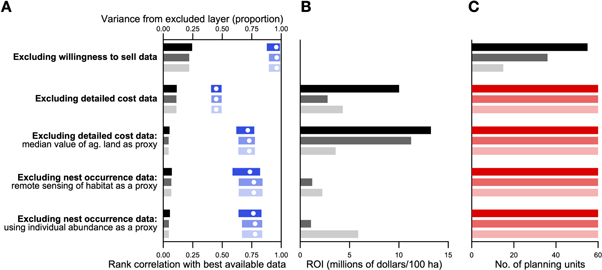
Figure 1. Comparisons between the scenario using the best available data and five scenarios that use reduced effort data. For all plots, lighter to darker colors correspond to the 33%, 66%, and 95% conservation goals, respectively. (A) Blue bars show the 95% confidence bounds for the correlations between the conservation value rankings produced by the best available data and the corresponding reduced effort scenarios listed on the left; white dots show means. Bars closer to zero have less correlation with the best available data, suggesting that obtaining better data has greater potential to improve planning efficiency. For each reduced effort scenario, the proportion of the uncertainty in estimating conservation value that is contributed by the excluded data layer is shown by grayscale bars—i.e. the lengths of the bars show by how much obtaining better data would increase the uncertainty bounds. (B) The cost savings, or return on investment (ROI), in terms of solution efficiency, of using data on nesting occurrence, high-resolution land cost, and likelihood of selling compared to the associated reduced effort scenarios listed on the left. (C) The minimum number of planning units needed to meet conservation goals for each scenario listed on the left. Solutions that did not meet conservation goals, despite incorporating all planning units in our planning region, are shown in red.
Download figure:
Standard image High-resolution imageContribution to uncertainty
The uncertainty within data layers, which can arise from estimation uncertainty (Wilson et al 2005, Rondinini et al 2006) or stochastic biological processes (Game et al 2008), is rarely incorporated into spatial planning (Lechner et al 2014). Uncertainty in conservation is ubiquitous and often substantial, however, and methods that explicitly aim to make the best decisions under uncertainty can lead to better outcomes (Game et al 2008). Quantifying how much uncertainty is added from each data layer can enable one to visualize the trade-offs between greater uncertainty and greater efficiency. To achieve this for each reduced effort scenario, we quantified the proportion of the uncertainty that is contributed by the excluded data layer as:

where N is the number of planning units, i, and CV is the coefficient of variation.
Return on investment through more efficient networks
Spatial planning with data that are more precise, accurate, or directly related to the target of interest presumably results in more efficient solutions for identifying the minimum set of land purchases required to meet a conservation goal. Given that conservation benefits are fixed, the difference in cost between solutions identified by the best available data versus reduced effort data is an intuitive and practically relevant index of the return on investment of obtaining better data. We calculated this measure by identifying, for each scenario, the minimum set of planning units that meets conservation targets for the least cost.
We identified minimum sets by sequentially choosing the planning unit with the highest conservation value until both conservation goals were met, recalculating the FOS after each step. We then estimated potential gains in efficiency from using the best available data compared to each reduced effort scenario as follows:

where BEST is the best scenario, RES is the reduced effort scenario,  is the minimum set identified using the best scenario,
  is the minimum set identified by the reduced effort scenario, and
  is the total extent of the targets, as estimated by the best scenario, that is contained within
  or
or 
Results
We found a trivially small cost savings when incorporating data on a landowner's likelihood of selling (figure 1(b)). Incorporating landowner likelihood of selling added the most estimation uncertainty (a mean of 22% of uncertainty in the conservation value estimates) and ignoring these data did not substantially affect rankings of conservation value or the efficiency of the minimum set of planning units needed to meet goals (figures 1, 2, S1). When likelihood of selling was ignored, which assumes that all land is available for protection, the minimum number of planning units needed to meet conservation goals varied from 18 for the least ambitious goal to 54 for the most ambitious (figure 1(c)). In contrast, for every scenario that includes likelihood of selling, not even protecting all land with likely sellers in every planning unit would be enough to meet goals (the bottom four scenarios in figure 1(c), shown as red bars).

Figure 2. The number of planning units, in a 10-unit window, that co-occur in matched windows for the rankings produced by the scenario using the best available data and each reduced effort scenario (shown for the 66% goal; results were not sensitive to how ambitious goals were). Solid lines show the mean number of shared planning units for the 10-unit moving window, and dotted lines show 95% confidence bounds. The highest ranked planning unit is marked with an O if it is the same for the reduced effort scenario and the best available data scenario, and marked with an X otherwise.
Download figure:
Standard image High-resolution image
Incorporating high-resolution land cost data had the largest influence on conservation value rankings (figure 1(a)), but also increased the variance of the uncertainty bounds by 11% (figure 1(a)). Ignoring costs altogether resulted in poor approximations of ranked conservation values (figure 1(a)). Using the median value of agricultural land as a proxy produced ranked conservation values that were better than those when ignoring costs, but rankings were still only about 70%–75% similar to those produced by the best scenario (figure 1(a)). The agricultural land cost data tended to rank planning units similarly to the better cost data for the highest value planning units, but dissimilarly for the lower value sites (figure 2). Ignoring land costs altogether resulted in dissimilar rankings across the entire range of conservation values (figure 2). Adding high-resolution land cost data also produced the greatest cost savings among the alternative scenarios: as much as $13 million/100 ha compared to using agricultural value and $10 million/100 ha compared to ignoring costs for the 95% goal (figure 2). Compared to ignoring costs altogether, using agricultural value improved conservation rankings, but produced less efficient minimum sets for the 66% and 95% conservation goals (figure 1(b)).
Using remotely-sensed habitat layers or individual abundance as proxies for nesting occurrence produced rankings that were only approximately 75% similar to those from the best scenario. The planning units identified as having the highest conservation value by these ecological data proxies were not the same as those produced by the best scenario, although all ecological datasets identified similar planning units as being of lowest conservation value (figure 2). The use of nesting occurrence data produced a greater cost savings ($6 million/100 ha) than high-resolution land cost data ($5 million/100 ha) for the 33% goal, but otherwise the savings from better ecological data were small compared to those from better cost data. The substantial savings from using nest occurrence data for the least ambitious conservation goal suggests that data on bird abundance alone do a poor job of identifying the highest priorities. This result is supported by low similarity between this scenario and the best scenario for the highest value planning units (figure 2).
Discussion
The cost savings for better land cost data were more than an order of magnitude greater than those for ecological data for the more ambitious conservation goals. This discrepancy suggests that if there are limited resources for data collection or if threats are so immediate that delaying conservation action could substantially worsen outcomes, as is true for our planning region (Field et al 2017b), obtaining better land cost data is likely to be the smarter investment. Incorporating landowner likelihood of selling (figure S3) drastically changed the outlook for whether it is possible to meet conservation goals, highlighting how the types of analyses here can also inform the likely effectiveness of conservation efforts.
Applying the framework presented here to other systems would facilitate the accumulation of evidence that could be used to find generalities about which types of data are likely to be most important for spatial planning in different social and ecological contexts. While the results of our case study were driven in part by region-specific factors, the key results are likely to apply to many regions and contexts. For example, we found that because land in coastal areas is costly, even small improvements in efficiency have the potential to lead to significant cost savings. Although exact comparisons are hard to make, each of our more detailed datasets was generated (including fieldwork and analysis) for ̃ US$ 200 000–300 000 and also produced substantial information gains toward other research questions beyond spatial planning. In contrast, estimated cost savings for many of the scenarios were in the millions of dollars, suggesting substantial return on investment.
Our results highlight the potential for large efficiency gains when using high quality cost data. This result has been found in previous studies that quantified sensitivity or importance of costs relative to biodiversity data (Carwardine et al 2010, Kujala et al 2018). Here, we show that the gains of investing in cost data also surpass data on likelihood of selling, which are rarely incorporated into planning, and a set of proxies for ecological data. The emerging generality of this pattern across different research approaches suggests that better cost data for conservation planning are likely to be a safe investment. We estimated costs by combining intensive data collection and a spatial regression model, an approach that is similar to hedonic pricing (e.g. Tyrväinen 1997). Other approaches to estimating costs might also be appropriate, including those that are similar (e.g. Carwardine et al 2010) and quite different (e.g. Withey et al 2012) from our method. Consequently, an emphasis on predicting spatial variation in conservation costs and covariation with targets (e.g. Ferraro 2003), akin to recent improvements in estimating species distributions (e.g. Guisan and Thuiller 2005, Zurell et al 2016), could greatly improve the effectiveness of spatial conservation planning (Armsworth 2014, Kujala et al 2018). In our example, the large savings provided by better cost data arose in part because the spatial resolution of the proxy for cost was low compared to the spatial resolution of the ecological proxies. We expect that the disparity in precision and accuracy between the best cost and ecological layers available for conservation planning will continue. The development of spatial cost layers typically does not receive the same degree of attention as the development of ecological layers (Kujala et al 2018), which can make use of increasingly high-resolution predictors (Pradervand et al 2014). Our results use a measure of return on investment, in terms of the costs of our conservation action of interest, purchasing land. The realized costs of conservation, however, often include opportunity (Adams et al 2010) and transaction costs (Ban and Klein 2009), as well as less tangible costs (e.g. Arponen et al 2010) such as the need for additional expertise and challenges associated with communicating with non-specialists. As understanding of these potential hidden costs improves, our general framework could be used as the basis for studies that further quantify the importance of overlooked costs in analyses of conservation problems.
For the analyses presented here, we compared reduced effort data against the best available data, which themselves are imperfect. Importantly, though, the data layers that we considered in the best scenario had robust uncertainty estimates, which we propagated by estimating conservation value across the full posterior distributions. By doing this, we also addressed the inherently uncertain nature of cost data (Carwardine et al 2010), which is a common source of criticism in conservation planning (Arponen et al 2010). While a key advance of our study was quantifying the uncertainty added by more complex data and analyses, further research could build on our results by focusing specifically on how complex datasets influence decision-making under uncertainty (e.g. Game et al 2008) or the consequences of using planning analyses and algorithms that do not easily propagate uncertainty (Lechner et al 2014).
We used the FOS index for our case study because it is well suited for both site prioritization and identifying minimum set solutions, and encourages a focus on return on investment, which is a powerful framework for determining conservation priorities (Naidoo and Ricketts 2006, Withey et al 2012). Our approach is not dependent on the spatial planning method, however. For example, our approach for estimating the cost savings of data layers could easily be replicated using popular tools such as Marxan (Watts et al 2009).
The generalizable aspects of our approach are also not limited to spatial planning problems. For example, we quantified how different aspects of data sources, including their accuracy, resolution, and uncertainty can influence the resulting decision-making. This more detailed approach is different from, but complementary to, recent approaches that address questions about the importance of different types of data using more generalized systems (Davis et al 2019) or mathematical derivations and simulations (Kujala et al 2018). Our approach simulates many of the real-world problems applied researchers and practitioners might face when conducting systems modeling or decision support analyses, especially as more methods incorporate uncertainty. Another key aspect of our approach was that we compared results using the best available data to results using typical datasets, or those that would be available in contexts for which analyses and planning must move forward using the best available data. These comparisons facilitate decision-making about the marginal benefit of additional data, which is often likely to be the quantity of interest, as few conservation problems are addressed with no data. Finally, looking at the return on investment of different types of knowledge in monetary terms has significant advantages for making sense of a complex set of options and facilitating efficient decision-making. For example, this framework allows direct comparisons of the cost of collecting better data to the savings, from network efficiency, of using better data. We believe that these features of our analysis will apply to most conservation problems, which are often interdisciplinary, urgent, and must be addressed with less than perfect information.
Acknowledgments
This work was funded by the National Socio-Environmental Synthesis Center (SESYNC), under funding received from the National Science Foundation (DBI-1052875a). Funding was also provided by the Connecticut Department of Energy and Environmental Protection and a Competitive State Wildlife Grant (U2-5-R- 1) via Federal Aid in Sportfish and Wildlife Restoration to the States of DE, MD, CT, and ME. Additional funding was provided by CT Sea Grant, University of Connecticut through Award No. NA14OAR4170086, Project Number R/SS-5. C. Field was funded by fellowships from the University of Connecticut College of Liberal Arts and Sciences Fellowship and a Robert and Patricia Switzer Foundation. This manuscript was greatly improved by comments from two anonymous referees.
Data availability statement
No new data were created or analyzed in this study