

Abstract
We present allometric-scaling relationships between non-point-source emissions of air pollutants and settlement population, using 3030 urban settlements in Great Britain (home to ca. 80% of the population of that region). Sub-linear scalings (slope < 1.0; standard error on slope ∼0.01; r2 > 0.6) were found for the oxides of nitrogen (NOx) and microscopic airborne particles (PM10 and PM2.5). That is, emissions of these pollutants from larger cities are lower per capita than would be expected when compared to the same population dispersed in smaller settlements. The scalings of traffic-related emissions are disaggregated into a component due to under-use of roads in small settlements and a fraction due to congestion in large settlements. We use these scalings of emissions, along with a scaling related to urban form, to explain quantitatively how and why urban airshed-average air pollutant concentrations also scale with population. Our predicted concentration scaling with population is strongly sub-linear, with a slope about half that of the emissions scaling, consistent with satellite measurements of NO2 columns over large cities across Europe. We demonstrate that the urban form of a particular settlement can result in the airshed-average air pollution of that settlement being much larger or smaller than expected. We extend our analysis to predict that the likelihood of occurrence of local air pollution hotspots will scale super-linearly with population, a testable hypothesis that awaits suitable data. Our analysis suggests that coordinated management of emissions and urban form would strongly reduce the likelihood of local pollutant hotspots occurring whilst also ameliorating the urban heat island effect under climate change.
Export citation and abstract BibTeX RIS

Original content from this work may be used under the terms of the Creative Commons Attribution 3.0 licence. Any further distribution of this work must maintain attribution to the author(s) and the title of the work, journal citation and DOI.
1. Introduction
About 4.3 million people die each year as result of outdoor exposure to particulate air pollution (data for 2015). In Europe, 520 000 excess deaths a year have been attributed to air pollution in 2017 [1] and in the megacity of London alone ∼10 000 people die each year from exposure to poor air quality [2] (data for 2010). These deaths are mainly due to exposure to nitrogen dioxide (NO2) and particulate matter (PM) of aerodynamic diameter less than 2.5 μm (PM2.5). In urban areas, the concentrations of both these pollutants are dominated by local traffic sources [3].
Half the world's population now lives in urban settlements; in highly developed countries such as the United Kingdom, more than 80% are urban dwellers [4], and these figures are predicted to rise. Although there have been major improvements in some aspects of urban air quality, for example very large reductions in sulfur dioxide and large particle pollution in London since the devastating 'smogs' of the 1950s and 1960s, some pollutants, including NO2 and PM (particularly PM2.5) remain intractable [5]. Technical solutions focused on tailpipe pollutant removal are controversial and subject to manipulation [6] and appear not to have yielded the desired or expected air quality improvements [1]. Hence, innovative ways of improving urban air quality are a global public health priority. The increasing focus on ecosystem services and natural capital [7, 8], green infrastructure [9, 10], and nature-based solutions [11] offers deposition of pollutants to vegetation and green space as a partial solution to urban air quality problems but we show below that it is not the most important aspect of urban form affecting air pollution except, arguably, at neighborhood-to-street scales. We follow Williams' definition of urban form [12]—i.e. the physical characteristics of settlements including the shapes, sizes, and arrangements of built elements. For our purposes, until we come to discuss pollution 'hot spots', urban form reduces to three urban metrics namely, total settlement area, adjustment of the synoptic wind, and adjustment of the boundary layer height. It has long been recognized that urban form affects pollutant emissions, through setting underlying patterns of land-uses and traffic-modes [13], a literature recently reviewed by Hankey and Marshall [14]. To the best of our knowledge, an emergent allometric pattern between urban form and air pollution concentrations has yet to be diagnosed. Our study is complementary to recent approaches which seek to simulate the development of canonical urban forms (i.e. dense cities, sprawl, etc) using agent-based approaches [15].
1.1. Scaling characteristics of cities
Many physical and socio-economic characteristics of urban areas scale with population [16], i.e. 'urban allometry' uncovers power-law relationships of the form:

where coefficient, Yj,o, and power-law exponent, αj, describe the scaling of characteristic Yj with some more commonly measured yardstick of 'scale' such as, in our case, population, P. Other yardstick measures, such as subsets of population [17, 18], GDP [19], or network fractal dimension [20], can be used if more appropriate to framing a particular study; we use population because it is a fundamental unit of social organization and to be consistent with prior work [21, 22]. The intention of allometric analysis is not to deduce causality, even regression-related Granger causality [23], but rather to search for simple emergent patterns in complex systems as an aid to understanding what is strictly contextual about instances of such systems and what holds more generally about them e.g. [24].
Sub-linear (αj < 1) scaling relationships indicate 'economy (or parsimony) of scale', as seen, for example, with road length and the volume occupied by urban infrastructure (pipes, cables, etc) [21, 24]. Super-linear (αj > 1) scaling relationships indicate 'increasing returns with scale' or 'scale-related excess', as is the case, for example, with incomes and the number of new inventions [25, 26]. Solid waste production from the world's current 27 megacities, and CO2 emissions from urban clusters in the USA, show super-linear scaling [18, 27]. Linear power laws (αj = 1 ± εj, where εj ≪ 1 is the error on the slope) include, for example, total employment and total housing of a city [16]; such linear relationships are neutral with respect to the distribution of population in one large city or several smaller urban settlements. When desirable traits scale super-linearly, or undesirable traits scale sub-linearly, the implication for policy-making is that organizing society into larger urban units can deliver improvements with respect to these traits. These scaling relationships prompt explanations in terms of a small set of basic principles that operate locally and describe the intrinsic socio-economic nature of urban living [16], in terms of parsimonious agent-based modeling [15], or via multiple regression model-finding of various kinds, e.g. [19, 28].
Here we extend the examination of the scaling behavior of urban settlements to include air pollution emissions and concentrations. When the scaling is robust, allometric scaling of pollution is a usefully emergent property of the complex urban system from which policy actions can be derived.
For evaluation of human exposure to air pollutants, the key metric is air pollutant concentration. In an urban area, air pollutant concentrations depend on imported background concentrations, local emission rates, atmospheric dilution and advection, chemical conversion, and local deposition, e.g. [29]. The likely scaling behavior of each of these influences on pollution concentrations is described below and in the SI, available online at stacks.iop.org/ERL/14/124078/mmedia. We begin with a focus on air pollutant emissions, which we would expect to be strongly related to population for a given level of economic development. Emissions inventories based on traffic flow, housing stock, and commercial activities are available for settlements of very different sizes across Great Britain (GB), which allows a detailed exploration of the scaling-law range across four orders of magnitude in population (102–106) and four orders of magnitude in urban area (1–103 km2) (see SI).
2. Methods
Our approach is to produce a GB analysis using appropriate national scale data. We look to minimize the impacts of using data from different sources captured at different scales by using high resolution (1 km) emissions data, urban boundaries, and road data from digital map data produced by the national mapping agency (OS, the Ordnance Survey of GB), alongside high resolution estimates of population from the UK's 2011 national census [30]. Population data were aggregated to output areas (the smallest mapping unit for the UK census). Settlement area and road length come from the OS Meridian2 product [31], and 2014 pollutant emissions at 1 km2 resolution are from the National Atmospheric Emissions Inventory [8] (see SI). Deriving settlement area from land-use, as we have done, rather than using designated metropolitan areas, allows us to consider many more urban areas and avoids the inclusion of large areas of sparsely populated land and low emissions within urban settlement boundaries and captures more of the fractality of urban areas [18, 20].
Six pollutants are considered initially: NOx, CO2, CH4, SO2, PM10, and PM2.5. Emissions from large industrial point sources, such as power stations, steelworks and oil refineries, were excluded, in order to focus on emissions related to urban structure, i.e. emissions from residential and commercial buildings and from transport sources. Standard model I ordinary least squares regression, with Log10Y dependent on Log10P, was used to derive power-law relationships; the square of the Pearson correlation coefficient, r, was used to determine goodness-of-fit [32]. Fits with r2 < 0.60 were considered statistically weak and excluded from further analysis.
3. Results
Five pollutants showed statistically well-defined (i.e. r2 > 0.6) sub-linear (α < 1.0) scaling with settlement population: NOx (α = 0.90 ± 0.01, figures 1(a) and S2); CO2 (α = 0.94 ± 0.01; figure 1(b)); PM10 (α = 0.72 ± 0.01; figure 1(c)); PM2.5 (α = 0.70 ± 0.01; figure 1(d)); and CH4 (α = 0.75 ± 0.01) (table S1). That is, emissions of these pollutants show an 'economy of scale/parsimony with scale', where 'scale' is measured by the settlement population and both emissions and population are aggregated within contiguous developed land use areas (see SI). This is broadly in line with previous results for CO2 emissions for cities in developed countries [33]. For SO2, the sub-linear relationship was statistically weaker (r2 < 0.6) (see section 2, and SI table S1, for details). In what follows we focus on NOx and PM, as urban pollutants with direct impacts on human health.
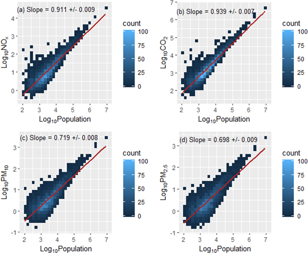
Figure 1. Allometric scaling of urban air pollution emissions, excluding those from large industrial point sources, in tonnes per year, for 3030 urban settlements in Great Britain, plotted as 2D log–log histograms against settlement population. Color shade represents the number of urban settlements per unit log10(population) per unit log10(emission) = 'count'. The best-fit straight line defines the power-law exponent (table S1). (a) Total NOx emissions. The equivalent scatter plot is provided in figure S2. (b) CO2. (c) PM10. (d) PM2.5.
Download figure:
Standard image High-resolution imageGiven that urban infrastructure [20, 21] and emissions both scale with population, it might be hypothesized that the scaling relationships for urban vehicle-derived air pollutant emissions against population would be the same as the relationship between road length and population. However, we find that the power-law exponent for NOx emissions against population (αNOx = 0.90 ± 0.01) is larger than the scaling of road-length versus population (αL = 0.69 ± 0.01; r2 = 0.84, sample n = 3024). This implies a significant loss of 'parsimony with scale' for pollutant emissions compared to the underlying infrastructure from which the emissions derive or, to put it another way, a significant change in the efficiency with which the road infrastructure is used in larger settlements compared to smaller settlements. The strength of this change in efficiency can be calculated by eliminating population from the two power-law equations. The resulting scaling relationship between NOx emissions and road length is substantially super-linear (α ∼ 1.3). This may be due to changes in the kinds of sources with settlement size, or due to 'under-use' of the transport infrastructure in small settlements and/or 'over-use' (congestion) in large settlements. We can distinguish between under-use and over-use by examining the variation of scaling with sample size.
4. Discussion
4.1. The sensitivity and robustness of scaling with respect to sample size
Figure 1 shows very strong positive skew and changes in the variance around the power-law best fit for different values of population, similar to that seen in other analyses using large samples of urban areas; see, for example, figure 4 in [18]. To test the sensitivity of our results to sample size, the power-law relationship (i.e. the value of αNOx) was re-calculated for sub-sets of the data, produced by removing more and more of the smaller settlements (figure 2).

Figure 2. The dependence of scaling power-laws with sample size. Power-law exponents α (top panel) and r2 coefficients of variance (bottom panel), for scaling correlations between NOx emissions and population (blue open circles) and between road length and population (red filled circles). Error bars for α show the standard error on the slope. Numbers in the bottom panel show the number of settlements used to generate each point. Each point on the graphs is calculated by removing all settlements in the dataset with population lower than the minimum given by the x-value of the point. The total population of the largest 3030 settlements in our complete dataset is 49.5 million. The scaling of emissions against road length for any subset of settlements (i.e. any value on the x-axis) is given by the ratio of alpha-values for emissions and road length shown in the top panel (as demonstrated in figure S3 in SI).
Download figure:
Standard image High-resolution imageThe power law exponent, αNOx, for the relationship between NOx emissions and population increases from 0.91 to 1.17 as smaller urban areas are progressively removed from the analysis. The peak value for αNOx occurs when 20% (∼600) of the settlements from the original sample of 3030 remain. This corresponds to when settlements of less than 5000 inhabitants are excluded. The other pollutants behave similarly. When sampling the 20–140 largest urban areas in Britain, the scaling relationship is stable and close to unity (figure 2; minimum populations 200 000 and 50 000, respectively). Applying a categorization to the urban settlements—e.g. 'industrial cities', 'commercial cities', etc [19]—has been applied to help diagnose scaling relationships in some settings; we have not been able to find a suitable categorization.
One might hypothesize that the NOx emissions scaling with population is entirely the result of road-length scaling with population in urban settlements. Comparing the population-scalings of NOx emissions and road length (figure 2), it is evident that the scalings start to converge for samples containing settlements with populations above about 5000. For any pair of scalings against population, the scaling of one with respect to the other is given by the ratio of the population scalings (see figures 2 and S3 in SI). When two scalings with respect to population converge to a common value, the scaling between the two parameters approaches unity (i.e. α ∼ 1, a linear scaling). The derived relationship between NOx emissions and road length diminishes (from ∼1.3 to 1.1, see caption to figures 2 and S3 in SI) when small settlements (populations < 5000) are removed. The NOx emissions scaling directly against road length stabilizes at ∼1.10, i.e. a 10% increasing pollution 'scale-related excess'. From this, we can deduce that it is a substantial change in source character or the relative 'under-use' of roads in small urban settlements that is the larger cause of the super-linear relationship between NOx emissions and road length for the whole sample of 3030 settlements, but that a substantial element due to congestion in larger settlements remains. The relationship between population and road length for the largest cities (rightmost point in figure 2) is similar to that found previously for cities in the USA (αL = 0.85) [21].
4.2. Airshed-average pollutant concentration scaling
The health effects of air pollution depend on exposure to pollution, and atmospheric pollutant concentrations are a much closer surrogate of exposure than emissions. To explore scaling relationships for pollutant concentrations and satellite-derived column densities, we examine the budget for an air pollutant in a well-mixed urban airshed, e.g. [29]
As discussed in more detail in the SI, C is the well-mixed airshed concentration of the pollutant, t is time, YE is the total city-wide emission rate of the pollutant per unit time, A is the area of the settlement (of length x), h is the atmospheric mixing height, Vd is the deposition velocity for the pollutant, C0 is the upwind concentration of the pollutant, u is the average wind speed across the urban area and through the height of the well-mixed boundary layer, p is the photochemical production rate of the pollutant, and L(C) is its chemical loss rate, which is a function of the abundance, C. We use this budget (equation (2)) to investigate the factors driving scaling properties of urban-airshed air quality in GB, not to model ground-level pollutant concentrations, a task for which many other more suitable but more complex models are available.
The steady-state pollutant concentration, Css, in the airshed is:
where k' is a pseudo first-order rate coefficient describing chemical loss, and so k'[C] is a simple proxy for L(C). The scaling behavior of equation (3) depends on the relative sizes of the terms in each parenthesis (see SI for a discussion of the influence of each term on allometric scaling). The simplest informative situation is where deposition is negligible, the pollutant is not formed or lost by chemical reaction in the atmosphere over the timescales of interest, and the upwind concentration is very much smaller than the concentration in the urban airshed. This simplification is appropriate for NOX and ultrafine aerosol (PM0.1), but not for PM2.5, for which primary emissions of particles [34] and transport of regional secondary aerosol, both contribute significantly to the ground-level urban concentrations [35]. The steady-state relationship then reduces to

Substituting population scaling for each variable into equation (4) suggests a heuristic for the overall scaling behavior of airshed average concentrations:

where αk is the power-law exponent against population for each of the parameters, k, in equation (4). One can think of this as a transformation of the pollution budget in physical space (equation (2) and more detailed continuity equations) into an equivalent budget in socio-economic 'space', in which population (or some other scale) provides the measuring yardstick. Equation (5) implies that the scaling of urban airshed concentration against population depends, therefore, on the relative magnitudes of the α parameters for the scaling of emissions, area, mixing height, and wind speed against population. Since the last three of these scalings depend crucially on urban form we can combine them into an urban form factor: αUF = αA/2 + αh + αu.
We have shown above how emissions scale with population: focusing on the largest 146 GB settlements (populations > 50 000), αNOx ∼1 (1.02 ± 0.03) for NOx emissions (figure 3(A), top-left panel). The equivalent power law relating settlement area to population in GB has αA ∼ 0.9 (0.88 ± 0.01; figure 3(A), center panel; note that −0.5 log(A) has been plotted, making the slope of the graph = −0.44). The power law generating αA relates the area of an urban settlement to its population; αA < 1 implies that urban area grows more slowly than in direct proportion to population (i.e. is a measure of the average extent of urban densification in the sample of settlements); while αA < 1 is a measure of the urban 'sprawliness' of the settlements). Although increased roughness and the urban heat island effect can cause mixing height, h, and wind speed, u, to change with settlement size [36], the changes are opposite in sign and approximately equal in magnitude (see SI). Hence, equation (5) simplifies to αC = αE – αA/2. So, the emergent pattern of pollution concentration as a function of urban population is the balance of emissions scaling and urban form scaling, with the former being about twice as important as the latter.
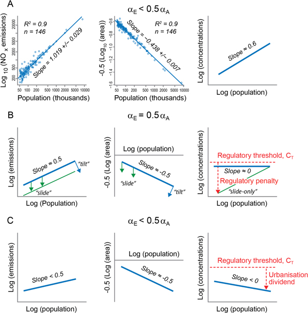
Figure 3. Expectations and opportunities afforded by urban scaling laws. Power-law relationships between total pollutant emissions and population (left column), settlement area and population (middle column) and airshed concentrations and population (right column), as posited by equation (5). (A) The current situation, showing data from 146 British settlements with populations >50 000, results in a concentration power-law slope of 0.55. (B) A scenario that aims to equalize pollutant concentrations everywhere below a regulatory threshold, CT, requires a serendipitous ratio of 2 between α for emissions and area with population. Environmental policies produce translation ('slide') or rotation ('tilt') effects on the scaling of key drivers. 'Slide-only' management interventions (green dashed line) to meet regulatory targets will penalize (red dashed line) populations in smaller urban areas. (C) Policy-making, cognizant of the tilt-and-slide effects of interventions, could be used to meet CT in the most cost-effective way, and actually deliver absolutely lower pollutant concentrations in large urban areas compared to smaller urban areas: an 'urbanization dividend'. To illustrate how key drivers influence the occurrence of local pollution hotspots (equation (7)), replace the scaling in the left-hand panels with that for YE/YL, in the middle panels that for YF, and in the right-hand panels that for YH, with due consideration for the power-law slopes discussed in the main text.
Download figure:
Standard image High-resolution imageSubstituting our results for how emissions and settlement area scale with population in GB gives a strongly sub-linear (αC = 0.55 ± 0.03), but still positive, scaling of pollutant concentrations with population (figure 3(A), top-right panel). This scaling is marginally larger than that of city-scale column-integrated airshed NO2, derived from satellite observations globally (αC = 0.48 ± 0.03) [22], as discussed further in the SI. The strongly sub-linear concentration scaling against population demonstrates that, in terms of the average behavior of the British settlements we examined, people living in large urban areas are much less impacted by urban airshed pollutant concentrations than would be expected if the emissions scaled linearly with population. This is not to say that some cities are more impacted by air pollution than others, either because of their deviation from the average picture or because of the existence of pollution 'hot spots'. We discuss both of these issues in turn, below, having first discussed the implications of the principal drivers for the general scaling behavior.
Equation (5) implies that there are three primary drivers that can aid understanding of urban airshed pollutant concentrations across a sample of urban settlements: (i) the scaling of emissions with population as a result of socio-economic patterns, only some of which are expressed spatially; (ii) the scaling of settlement area with population, usually referred to as 'urban density' or its converse, 'sprawl'; and (iii) the scaling of meteorological factors with population as a result of socio-economic patterns expressed in those elements of urban form that affect aerodynamic roughness (e.g. heterogeneity in building height) and the surface energy balance. Because of their tendency to cancel, the scaling of meteorological factors is only effective insomuch as the magnitude of the scaling of mixing height, αh, becomes different from that for wind speed, αu, conditions that are not simple to envisage.
Retaining the deposition parameter in the simplification of steady-state equation (3) produces

in which the scaling will depend on the relative size of the terms in parentheses in the denominator. The deposition term in this boundary-layer budgeting approach is much less than 10% of the u.h term for all but the largest (A ≈ 100 km2) conurbations (see SI). Even for these large urban areas, deposition will have a minor influence on the steady-state airshed concentration and on the scaling of those concentrations with population. The effect of expanding urban green infrastructure at the airshed scale will likely be much stronger through its effect on urban form, especially total urban area (equation (4), above) [37]. The effects of vegetation on surface roughness and, hence, the mean wind speed, u, and the effects of roughness and local heat balance on the mixing height, h [36, 38], will be more influential on urban airshed-average pollution concentrations than the effect of deposition on vegetation (see [39] and similar approaches which focus solely or mainly on the deposition term). However, at the local scale, the effect of green infrastructure on pollutant concentrations is a context-dependent balance of fumigation and deposition effects with potentially large impact [10, 38, 40, 41].
4.3. The relative importance of emissions and urban form for individual settlements
Calculating the residual between the point for each settlement and the scaling best-fit line (see SI) provides a measure of the degree to which each settlement is doing relatively 'better' or 'worse' than expected, based on the overall allometry [24]. Figure 4 shows residuals for the 146 largest GB settlements, ranked by their NOx emission residual (red line), calculated such that a positive residual represents a better than expected (i.e. lower) emission than predicted by the allometric relationship with population.

Figure 4. Ranking settlements with respect to their deviation from the scaling relationship of NOx with settlement population. The 146 largest British settlements are ranked by their NOx emission residual (red line), calculated such that a positive residual represents a 'better than expected' (i.e. lower) emission than predicted by the allometric correlation. Superimposed on the graph are the combined residuals for the emission and settlement area scalings against population (blue line), where positive residuals are 'better than expected' areas for a given population.
Download figure:
Standard image High-resolution image
Superimposed on figure 4 are the combined residuals for emissions and settlement area scaling against population (blue line). Where the blue line is more positive than the red line in figure 4, the relevant settlement benefits more than expected from its urban form, making settlements that are doing better than expected on the basis of emissions (the left-hand side of figure 4) do even better, and ameliorating the 'worse than expected' performance for settlements that are doing worse than expected on the basis of emissions (the right-hand side of figure 4). Where the red line is less positive than the blue line, the situation is reversed: urban form makes the performance of individual settlements worse than expected on the basis of emissions alone. The top 20 and bottom 20 settlements whose concentration ranking is most changed by the urban form factor, compared to an emissions-only ranking, are listed in table S2 of the SI. The city whose rank is most improved by urban form is the post-world-war-2 'garden city', Milton Keynes. Of the largest British cities, Birmingham, Manchester, Glasgow, and Sheffield are in the top 20 'most improved by urban form', whereas London is largely unchanged.
4.4. The expected scaling of air pollution hotspots
Not all pollution is well-mixed throughout the urban airshed. Pockets of high concentration exist, particularly in poorly ventilated street canyons through which high volumes of traffic flow [10, 38, 41, 42]. We expect the likelihood of the occurrence of pollution hotspots, H, to be

where F is the fraction of roads liable to poor ventilation (fumigation), and YE/YL is the average emission per unit road length in the urban area.
We have shown above that road length is a stronger and stronger linear predictor for NOx emissions as GB urban areas increase in size, but that a ∼10% pollution scale-related excess persists, presumably as a result of increasing congestion in the largest settlements. The scaling of F with population will depend on changes in urban form [42]. Some changes in urban form with scale—e.g. the emergence of an increasingly dense and increasingly high-rise central business district—will generate a larger fraction of poorly ventilated streets. Strict self-similarity (i.e. 'tiling' of urban form) would suggest that, neglecting any wind speed scaling as discussed in the SI, F scales linearly with population (i.e. we expect αF ≥ 1). Overall, then, we deduce that, as cities grow, local traffic-related air pollution problems become exacerbated super-linearly (i.e. the scaling of H with population, αH ≥ 1.1). Engineered solutions to urban air pollution hotspots could focus, therefore, on changes to urban form that reduce the fraction of poorly ventilated urban areas until traffic emissions are sufficiently reduced. Since the same canyon-like urban forms trap heat as well as pollutants [36, 43, 44], and so contribute to the urban heat island, any changes in urban form made to ameliorate air pollution hotspots will have the co-benefit of relieving urban heating (itself a phenomenon with undesirable human health impacts [45]).
5. Conclusions
The results above offer the prospect of 'scale-aware policy tools'. The right-most panel of figure 3(B) shows a scenario that broadly reflects current air quality policy for cities in developed countries, which has the general aim of bringing pollutant concentrations everywhere below a critical threshold, CT, defined by environmental regulation. Equalizing pollutant concentrations across urban areas of all sizes implies a serendipitous canceling of the values of α for both emissions and the urban form factor with population. Only in the special case of αE = αUF/2 would urban airshed concentrations become independent of population. The bottom panels (figure 3(C)) show that, when αE < αUF/2, achievable by increasing αUF and decreasing αE for instance, pollutant concentrations begin to scale negatively with population. In such an eventuality, large urban areas would have airshed pollutant concentrations that would be absolutely lower than those in smaller urban areas, rather than simply being better than expected (i.e. pollutant concentrations would scale negatively rather than sub-linearly with population, resulting in an 'urbanization dividend', see figure 3(C), bottom-right panel). Policy-making should recognize this urban allometry, and emissions and the urban form factor should be managed accordingly.
Therefore, the scaling properties of the key drivers of urban air pollution offer policy-makers a new way of categorizing and conceptualizing their approaches to improving urban air quality. Proposed interventions can immediately be categorized in terms of their ability to modify urban airshed concentrations and the likelihood of pollution hotspots. Further, it is possible to decide whether such interventions predominantly 'tilt' (i.e. reduce the value of αj in equation (1)) or 'slide' (i.e. reduce Yj,o while αj remains unchanged) the scaling of the key driver on which they act. Interventions that tilt the scaling of a key driver by acting on the largest urban areas will be the most cost-effective because (i) they will act on the largest populations first; (ii) the regulatory burden will not fall unduly on smaller urban areas which already do better in absolute terms of air quality; (iii) such interventions will simultaneously improve urban airshed concentrations and lessen the likelihood of hotspots; and (iv) innovation will tend to cascade to smaller scales bringing, in time, a translation towards improved air quality everywhere.
'Decoupling' emissions from population, such that αE < 0.5, can be achieved by extraordinary investment in public mass transport, electrification or exclusion of vehicles, low- or zero-emissions zones, etc, starting with the largest urban areas but not focusing exclusively on the single largest city (as discussed in the SI, London already does 'better than expected' being ranked 21 out of 146 largest settlements in GB in terms of its emissions residual). Engineering population densities so that αA > 1 would mean slowing or avoiding the trend of densification with growth while not increasing per capita emissions, by interleaving dense urban areas well served by mass public transport with areas of green space, for instance. Changing the urban-area scaling with respect to population will have many impacts on city metabolism, so that any engineering of αA needs to be undertaken with care for trade-offs with other urban processes and resource demands. Alternatively, as cities grow and become denser it will be essential that the desirable scaling of emissions with population tilts even further. Taken together, these measures could deliver absolutely lower pollutant concentrations in large urban areas and therefore substantial public health benefits. Moreover, equation (7) suggests that this kind of coordinated management of emissions and urban form would strongly reduce the likelihood of local pollutant hotspots occurring and also ameliorate the urban heat island effect. The deliberate engineering of aerodynamics and deposition sinks—e.g. through nature-based solutions—can have only a small effect on airshed concentrations, except in very carefully designed locations [10, 40], but can substantially influence dispersion and so reduce local air pollutant concentrations that way [38], whilst being socially desirable for many other reasons [46].
Acknowledgments
This work was funded in part by the UK Engineering and Physical Sciences Research Council's Sustainable Urban Environment II programme (EP/F007426/1); we thank Professor Chris Rogers (University of Birmingham) and Professor Rachel Cooper (Lancaster University) for programme leadership and our many programme colleagues for insightful interdisciplinary collaborations. A R M K acknowledges further funding support from the Natural Environment Research Council (NE/N003195/1, NE/S00940X/1, NE/S00582X/1, NE/S013814/1, NE/S003487/1). This is paper number 10 of the Birmingham Institute of Forest Research.
Author contributions
A R M K and C N H conceived the study and obtained funding; M J B extracted data and tested scaling relationships; J D W led GIS data extraction with support from G D; A R M K, C N H and J D W directed the data analysis; A R M K, M J B, J D W and C N H wrote the paper collaboratively.
Author information
The authors declare no competing financial interests. Correspondence and requests for material should be addressed to ARMK at .
Data availability statement
The data that support the findings of this study are openly available at DOI: 10.25500/edata.bham.00000384.