

Abstract
Cities typically exhibit higher air temperatures than their rural surroundings, a phenomenon known as the urban heat island (UHI) effect. Contrasting results are reported as to whether UHI intensity (UHII) is exacerbated or reduced during hot weather episodes (HWEs). This contrast is investigated for a four-year period from 2015 to 2018, utilising a set of observational data from high-quality meteorological stations, as well as from hundreds of crowdsourced citizen weather stations, located in the urban region of Berlin, Germany. It can be shown that if HWEs, defined here as the ten percent hottest days or nights during May–September, are identified via daytime conditions, or by night-time conditions at inner-city sites, then night-time UHII is exacerbated. However, if HWEs are identified via night-time conditions at rural sites, then night-time UHII is reduced. These differences in UHII change can be linked with prevalent weather conditions, namely radiation, cloud cover, wind speed, precipitation, and humidity. This highlights that, beside land cover changes, future changes in weather conditions due to climate change will control UHIIs, and thus heat-stress hazards in cities.
Export citation and abstract BibTeX RIS

Original content from this work may be used under the terms of the Creative Commons Attribution 3.0 licence. Any further distribution of this work must maintain attribution to the author(s) and the title of the work, journal citation and DOI.
1. Introduction
During the last few decades, near-surface air temperature (T) as well as heat extremes have increased worldwide (Alexander et al 2006, Perkins et al 2012, Russo et al 2014). Hot weather episodes (HWEs) adversely affect human health, different societal sectors, and ecosystems (Smoyer-Tomic et al 2003, Ciais et al 2005, García-Herrera et al 2010). Concurrently, ongoing worldwide urbanization puts more and more people under risk of being adversely affected by elevated T, as cities typically show higher T than rural surroundings, a phenomenon known as the 'urban heat island' (UHI) effect (Oke 1982, Arnfield 2003). With projected future increase in frequency, duration, and intensity of heat waves globally (Meehl and Tebaldi 2004, Fischer and Schär 2010, Russo et al 2014), as well as projected ongoing urbanization (United Nations 2015), the question whether UHI intensities (UHIIs) are exacerbated during such episodes is of high relevance for risk assessment. Beside influences of size, morphology, and contiguity of each city onto UHIIs, both in air as well as surface temperatures (Arnfield 2003, Debbage and Shepherd 2015, Zhou et al 2017), UHIIs are largely determined by weather conditions, with dry, clear, and calm conditions favouring large UHIIs (Morris et al 2001, Kim and Baik 2005, Erell and Williamson 2007, Arnds et al 2017, Beck et al 2018).
At first glance, seemingly contradictory results concerning effects of heat waves, or more generally, HWEs, onto UHIIs are reported. While some studies show increasing UHIIs (Fenner et al 2014, Li et al 2015, Founda and Santamouris 2017, Ramamurthy and Bou-Zeid 2017, Zhao et al 2018), others reveal unchanged or even reduced UHIIs (Zhou and Shepherd 2010 , Scott et al 2018, Rogers et al 2019). Several reasons have been put forward to explain these results, mainly relating them to changes in weather conditions, such as increased radiative input or altered wind patterns (Li et al 2016, Founda and Santamouris 2017, Sun et al 2017, Scott et al 2018). These in turn lead to changes in the urban and rural energy balance (Li et al 2015, Ramamurthy and Bou-Zeid 2017, Sun et al 2017, Zhao et al 2018). Since most of these studies applied different methods to identify the subsequently analysed HWEs, it could be hypothesized that the contrasting results are at least partly due to the application of different methods to identify these episodes. The definition of heat waves, as well as whether they are identified at an urban or a rural location, can substantially affect their frequency, duration, and long-term trends (Fenner et al 2019). Further, it could be hypothesized that by applying different methods, both increased and decreased UHIIs during HWEs can be detected, even for a single city.
One common weak aspect of observational UHI studies is the use of only one pair of or very few measurement stations, as they might not be representative for the whole city. A novel approach using low-cost weather stations or citizen weather stations (CWSs) at up to several hundreds of sites for one city, located in various urban settings, has shown great potential and applicability (Wolters and Brandsma 2012, Schatz and Kucharik 2015, Fenner et al 2017, Meier et al 2017, Scott et al 2017). Crowdsourcing of CWS data is an inexpensive option to collect substantial amounts of atmospheric data (Muller et al 2015), also enabling investigations in regions where high-quality data are missing or sparse.
To shed more light onto the aspect of contrasting results concerning UHII changes (∆UHIIs) during HWEs, the overarching aim of this study is to systematically investigate how the choice of location and time of day to define HWEs might lead to contrasting results. Specifically, the hottest days and hottest nights during May–September during the years 2015–2018 are investigated for the urban region of Berlin, Germany, and put into contrast to the rest of the days/nights. This is done by identifying these episodes separately in rural and the most densely built-up urban locations to investigate the influence the location for identification can have onto results. A data set of a multitude of high-quality meteorological observations from reference stations (REFs) as well as quality-controlled crowdsourced data from nearly 2000 CWSs are utilised. Moreover, it is then analysed how possible contrasts in ΔUHIIs are linked to differences in weather conditions. In view of climate change, it is important to understand present-day mechanisms for altered UHIIs, as future climate might change frequency, duration, and intensity of different types of weather conditions, and thus UHIIs.
2. Data and methods
2.1. Study area and period
This study focuses on the mid-latitude city of Berlin and surrounding region (Köppen–Geiger classification Cfb—humid warm temperate climate, Kottek et al 2006). Berlin is Germany's largest city with nearly 3.5 million inhabitants by the end of 2015, located in the eastern part of the country (52.52° N, 13.40° E). The city spreads over an area of 892 km2 with approximately 35 km in north–south and 45 km in east–west direction. The city's topography is relatively flat with solitary hills at the edge of the urban agglomeration. Agricultural lands and forests surround the city. Inner-city areas mostly consist of compact and open midrise building structures (Local Climate Zones—LCZs 2 and 5, Stewart and Oke 2012), surrounding these are mainly open low-rise detached housing areas (LCZ 6) and forests (LCZ A) (Fenner et al 2017). The study period covers four years from 2015 to 2018, analysing the months May–September.
2.2. Meteorological data and processing
Two sets of near-surface T data were used for the characterisation of UHII: data from high-quality reference stations (REFs) and crowdsourced CWSs (figure 1). The network of REFs consists of 51 stations maintained by the German Meteorological Service (Deutscher Wetterdienst—DWD), the Institute of Meteorology at Freie Universität Berlin (FUB), and the Chair of Climatology at Technische Universität Berlin (TUB). T is measured in 2 m above ground level at all sites, except for three stations (see supplementary table S1, available online at stacks.iop.org/ERL/14/124013/mmedia). DWD data are available as quality-checked products at hourly resolution (DWD Climate Data Center 2018). Data at FUB stations are available at five-minute resolution, at TUB stations at one-minute resolution. Both were aggregated to hourly mean values (time stamp at the end of averaging interval) after quality control (QC). QC of FUB and TUB data was carried out as in Meier et al (2017) with additional filters for spikes and persistence. A visual inspection and removal of remaining implausible values was performed after automatic QC.
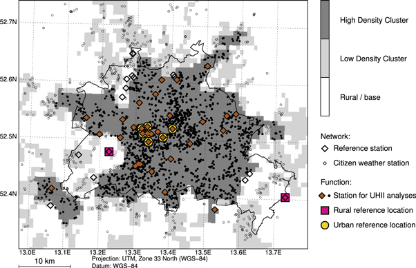
Figure 1. Location of weather stations in the Berlin region during 2015–2018. Stations that are used in the urban heat island intensity (UHII) analyses are located within High Density Cluster. Data at rural reference locations are used for calculation of each station's UHII and identification of rural hot weather episodes (HWEs), data at urban reference locations are used for identification of urban HWEs. The black line marks the city border of Berlin. Classification of urban clusters based on Global Human Settlement product 'GHS S-MOD' (Pesaresi and Freire 2016).
Download figure:
Standard image High-resolution imageData from CWSs of the 'Netatmo' company (https://netatmo.com) were collected via the company's application programming interface, retrieving instantaneous values at hourly intervals at all available stations for each hour during the study period. A full description of the methods to collect, store, and process CWS data can be found in Meier et al (2017). Deviating from Meier et al (2017), CWS data in this study were assigned to the nearest full hour. For QC, the statistically-based methods of 'CrowdQC v1.2.0' (Grassmann et al 2018, Napoly et al 2018) were applied, which are independent of reference T data. Quality-controlled CWS data at level O1 (see Napoly et al 2018) were used in all analyses.
Only stations (REFs and CWSs) with ≥80% valid hourly data in at least one year (May–September) were included. Data from all stations were corrected for height differences to a reference height of 45 m above mean sea level with the dry adiabatic lapse rate (−9.8 × 10⁻³ K m−1), using elevation data from the Shuttle Radar Topography Mission version 4.1 (Jarvis et al 2008), as described in Fenner et al (2017).
For characterization of weather conditions, meteorological data at seven sites were used (supplementary table S2, supplementary figure S1). These sites are located throughout the urban region of Berlin to describe conditions representative for the whole region. Hourly data of 2 m relative humidity, 2 m surface air pressure, cloud cover fraction, 10 m wind speed, precipitation, and downwelling shortwave and longwave radiation were used (supplementary table S2). For each variable a synthetic time series as the arithmetic mean across all available sites was calculated. Specific humidity was calculated per site on the original temporal resolution of one hour using site-specific relative humidity, surface air pressure, and T, and then averaged across all available sites.
2.3. Site selection for UHII analyses
All REFs and CWSs that are located within High Density Cluster of the Global Human Settlement Layer product 'GHS S-MOD' (Pesaresi and Freire 2016) were selected (figure 1) to represent climate conditions of the built-up environment of Berlin. A total of 33 REFs and 1945 CWSs for the investigated four years were available.
'Rural' sites to calculate each site's UHII (see next section for definition) were selected based on the mapping of LCZs as carried out in Fenner et al (2017). The two available REFs located in LCZ B 'scattered trees' were selected as rural reference locations (figure 1, supplementary table S1). These two sites have no buildings in their local-scale surroundings, LCZ B provides the 'most rural' T signal among LCZs in the region of Berlin (Fenner et al 2017), and hence the sites are highly suitable for UHII calculation (Fenner et al 2014, 2017). A synthetic rural time series was calculated as the arithmetic mean of the rural sites if both stations provided valid data, otherwise set to missing value. This synthetic rural time series was also used to identify rural HWEs (see section 'Definition of HWEs').
Further, an 'urban' synthetic time series was derived analogously to identify urban HWEs. For this, all REFs falling into the 'most urban' LCZ class 2 'compact midrise' were selected (figure 1, supplementary table S1) and the arithmetic mean across all sites was calculated if at least two stations provided valid data.
2.4. Calculation of UHII and its temporal deviations
Firstly, hourly T differences between each station (REFs and CWSs) and the synthetic rural time series were calculated, referred to as UHII for each station.
Secondly, UHII for each station was aggregated to an arithmetic mean value for daytime (13–16 h UTC + 1) and night-time (01–04 h UTC + 1) intervals each day. UHII was analysed separately for daytime and night-time periods, as it shows a distinct diurnal cycle with largest UHIIs at night (Oke 1982, Chow and Roth 2006, Erell and Williamson 2007, Fenner et al 2014, Beck et al 2018). A discussion on the selected time intervals and study period is given in supplementary Discussion D1. Mean UHII for each interval at each day was only calculated if at least three hourly values per interval were available, otherwise set to missing value. Analogously, mean T during daytime (Tdaytime ) and night-time (Tnight-time ) intervals for the synthetic rural and urban time series were calculated.
UHII change (∆UHII) during HWEs (see next section for definition) was derived for each station as follows. For daytime and night-time UHII, the arithmetic mean value of UHII during 'normal' days, i.e. all days not identified as HWEs, and the arithmetic mean of UHII during HWEs was calculated for each station. Then, each station's ΔUHII was calculated as the difference between mean UHII during HWEs and mean UHII during normal conditions.
2.5. Definition of HWEs
The 10% hottest days and hottest nights during May–September were investigated, identified separately using the synthetic rural and urban reference time series. These days and nights are referred to as 'rural hot days/nights' and 'urban hot days/nights' (n ≈ 61), and put into contrast to the rest of the days/nights, referred to as 'normal conditions'. The term 'hot weather episodes' is used in this study to refer to these episodes instead of 'heat waves', as they may occur as single days/nights, which are regarded as being too short to count as a heat wave.
A rural (urban) hot day was identified if a day had Tdaytime > 90th percentile of the probability density function of Tdaytime during the four years (May–September) of the synthetic rural (urban) time series (thresholds: rural 29.1 °C, urban 29.2 °C). Similarly, rural (urban) hot nights were identified, but using Tnight-time (thresholds: rural 17.4 °C, urban 20.9 °C). More details on the choice of this definition is given in supplementary Discussion D2.
In this study, each day starts at 05 h (UTC + 1) and ends at 04 h (UTC + 1), hence the night-time interval covers the last 4 hours of each day. Hot days (identified via the daytime interval) thus have a night-time interval following the daytime interval, while hot nights (identified via the night-time interval) have a preceding daytime interval before the night-time interval.
2.6. Statistical tests
Statistical significance of ΔUHII and the difference in weather conditions was tested applying the non-parametric Mann-Whitney-U test (Mann and Whitney 1947). Sample distributions consisted of mean UHII of each station during HWEs and normal conditions, respectively (for ∆UHII), and of the mean value across all sites per analysed variable (for weather conditions) during HWEs and normal conditions. Statistical significance of the test statistic U was evaluated using a two-sided p-value. Statistical significance was set at p ≤ 0.05. Since sample distributions of REFs and CWSs differ considerably, and hence also variance between the networks (e.g. figure 2), an effect size of the mean difference in UHII between normal conditions and HWEs was calculated for each network. Cohen's d (Cohen 1988) as a descriptor for effect size between data sets a and b was calculated:

with mx being the mean of data x (x = a or x = b) for nx = sample size of x:

and the pooled standard deviation σ:

where sx = standard deviation of data x:

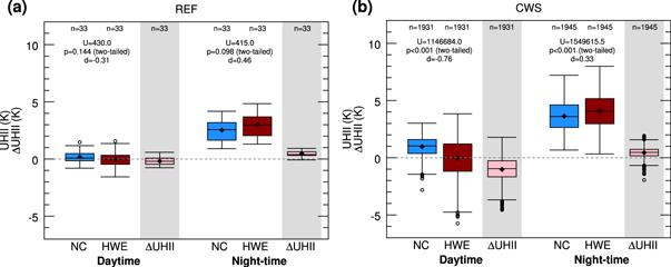
Figure 2. UHII and UHII change (∆UHII) during normal conditions and rural hot days during 2015–2018, May–September. UHII quantification using (a) high-quality reference stations (REFs) and (b) citizen weather stations (CWSs) during daytime (13–16 h UTC + 1) and night-time (01–04 h UTC + 1). Each box contains temporal mean values of each station, the Mann-Whitney-U test was applied to determine statistical significance of difference in UHII between normal conditions (NC) and hot weather episodes (HWE). Effect size of mean differences was determined using Cohen's d. The number of stations providing valid data is displayed above each box. Boxes range from 1st to 3rd quartile, median is denoted as horizontal line, mean as diamond, whiskers indicate 1.5 fold inter quartile range from upper and lower boundary, or the maximum and minimum, respectively. Values outside that range are displayed as circles.
Download figure:
Standard image High-resolution imageEffect size is described as very small (∣d∣ ≤ 0.2), small (0.2 < ∣d∣ ≤ 0.5), medium (0.5 < ∣d∣ ≤ 0.8), or large (∣d∣ > 0.8) (Cohen 1988).
3. Results and discussions
3.1. Effects of hot days onto UHII
Average UHIIs during normal conditions and rural hot days are displayed in figure 2, showing generally reduced daytime UHII during hot days. The change in mean UHII is insignificant for REFs with a small effect size (−0.18 K, p = 0.144, figure 2(a)), but medium in size and highly significant for CWSs (−1.02 K, p < 0.001) (figure 2(b)). Half of the REFs exhibit a negative UHII (sometimes called 'urban cool island', i.e. lower T within the city as compared to its surroundings), during normal conditions as well as during hot days (figure 2(a)). Contrastingly, only 13% of CWSs (=265 stations) show a negative UHII during normal conditions (figure 2(b)). This contrast is likely due to differences in station locations between REFs and CWSs, the latter being located closer to buildings compared to more open locations of REFs, leading to higher T being measured (Fenner et al 2017). Negative UHIIs have previously been reported for Berlin (Fenner et al 2014) and other cities (e.g. Runnalls and Oke 2000, Chow and Roth 2006, Fortuniak et al 2006, Erell and Williamson 2007), as well as even more negative UHIIs during HWEs (Fenner et al 2014, Rogers et al 2019). The large spread in UHIIs and ∆UHIIs (figure 2) highlights that individual stations might respond differently to hot weather conditions due to respective site characteristics (Zhou and Shepherd 2010, Scott et al 2018), underlining the benefit of analysing many stations within one city. In this respect, CWSs complement existing station networks in cities, as the large number of CWSs and the variety of urban settings in which they are located enables observations of the large spatial heterogeneity of urban T (Fenner et al 2017).
Contrasting to our results and those found for other cities (Rogers et al 2019), some studies showed amplified daytime UHIIs during HWEs (Schatz and Kucharik 2015, Founda and Santamouris 2017, Zhao et al 2018). Anthropogenic heat release from air-conditioning (AC) systems into the urban atmosphere contributes to UHIIs (Ohashi et al 2007, de Munck et al 2013), and thus, increased heat output of such systems during HWEs promotes increased UHIIs (Schatz and Kucharik 2015, Zhao et al 2018). Note that in Berlin AC of households is uncommon and that space heating, which could contribute to increased UHIIs, is most likely not used during HWEs during May–September. If an influence of space heating was present in the data of normal conditions, ∆UHII would be even more distinct if the influence of this heat output was removed. Further, only few sites are located in commercial areas where AC systems are more common, hence their influence onto the presented results is small. Overall, the influence of anthropogenic heat onto near-surface T is regarded as marginal for the analysed data in Berlin. Other studies relate increased daytime UHIIs during HWEs to changes in wind patterns (Founda and Santamouris 2017, Ramamurthy and Bou-Zeid 2017), while still others find that such changes cannot explain altered UHIIs (Rogers et al 2019).
During night-time of rural hot days, CWSs show a significant mean increase in UHII of 0.45 K (p < 0.001), while mean ∆UHII of 0.47 K for REFs is not significant (p = 0.098) due to the much smaller sample size (figure 2). This finding highlights, firstly, good agreement between both station networks, secondly, the benefit of CWSs in terms of sample size, and lastly, adds further evidence to existing studies, showing the intensifying effect of hot daytime weather onto night-time UHIIs (Fenner et al 2014, Li et al 2015, Schatz and Kucharik 2015, Sun et al 2017, Zhao et al 2018).
As opposed to normal conditions, the analysed rural hot days are characterized by significantly higher radiative shortwave and longwave energy input, lower cloud cover fraction and decreased wind speed during the day, and overall increased atmospheric humidity (figure 3, table 1). The precipitation amount and the days with precipitation are also reduced compared to normal conditions. Such weather conditions favour spatial T differences and lead to pronounced night-time UHIIs (Runnalls and Oke 2000, Morris et al 2001, Kim and Baik 2005, Erell and Williamson 2007, Arnds et al 2017, Fenner et al 2017, Beck et al 2018). With significantly decreased daytime and unchanged night-time wind speed, increased daytime radiation during hot days induces more daytime sub-surface heat storage and subsequent night-time heat release, leading to positive ∆UHII (Hamdi et al 2016, Sun et al 2017, Zhao et al 2018).

Figure 3. Weather conditions during rural hot days and normal conditions during 2015–2018, May–September, (a) downwelling shortwave radiation (rsd), (b) downwelling longwave radiation (rld), (c) cloud cover fraction (cc), (d) wind speed (ws), (e) precipitation (prcp), (f) specific humidity (hus). Percentiles for shading correspond to the respective probability distribution function during hot days and normal conditions. Measurement data from seven sites used (see section 2.2, supplementary figure S1, supplementary table S2), averaged across available sites.
Download figure:
Standard image High-resolution imageTable 1. Mean differences (∆) in weather conditions between hot weather episodes (HWEs) and normal conditions (NC) during 2015–2018, May–September. rsd: downwelling shortwave radiation, rld: downwelling longwave radiation, cc: cloud cover fraction, ws: wind speed, hus: specific humidity, prcp: precipitation. The Mann-Whitney-U test was applied to determine statistical significance (not for precipitation), significant differences (p ≤ 0.05) are marked as bold numbers. Measurement data at seven sites used (see section 2.2, supplementary figure S1, supplementary table S2), averaged (sum for precipitation) across hours of daytime (13–16 h UTC + 1) and night-time (01–04 h UTC + 1) intervals, and across available sites.
| Identification location | Urban | Rural | ||||||
|---|---|---|---|---|---|---|---|---|
| Hot weather episode | Hot days | Hot nights | Hot days | Hot nights | ||||
| Analysis interval | Daytime | Night-time | Daytime | Night-time | Daytime | Night-time | Daytime | Night-time |
| ∆rsd (W m−2) | 172.4 | — | 156.7 | — | 171.1 | — | 92.4 | — |
| ∆rld (W m−2) | 36.7 | 34.4 | 35.0 | 38.4 | 34.2 | 29.7 | 35.1 | 44.0 |
| ∆cc (octas) | −2.1 | −0.6 | −1.7 | −0.5 | −2.2 | −0.9 | −0.6 | 1.2 |
| ∆ws (m s−1) | −0.7 | 0.2 | −0.7 | −0.1 | −0.7 | 0.1 | 0.0 | 0.6 |
| ∆hus (g kg−1) | 1.6 | 2.6 | 1.9 | 2.8 | 1.6 | 2.4 | 2.5 | 3.3 |
| ∆prcp (mm), % days with prcp (HWE/NC) | −0.3, 1.6/22.9 | −0.1, 16.1/14.5 | −0.3, 4.8/22.5 | −0.1, 17.7/14.4 | −0.3, 3.3/22.7 | −0.1, 11.5/15.1 | 0.1, 11.7/21.7 | 0.2, 28.3/13.2 |
As a further consequence of strong daytime radiative forcing during HWEs, turbulent mixing over a deep planetary boundary layer leads to small differences between urban and rural T (Bohnenstengel et al 2011, Wouters et al 2013). As a result, the choice of location to identify hot days has negligible effects onto results concerning UHII (see supplementary figure S2). Most of rural and urban hot days (54 out of 61/62, = 88/87%) are identical (supplementary figure S3a). Further, threshold temperatures to identify them are similar (rural: 29.1 °C, urban: 29.2 °C), as are changes in weather conditions (table 1) with no significant differences between rural and urban hot days for any of the analysed weather variables (not shown).
3.2. Effects of hot nights onto UHII
When hot nights are identified at urban locations (figures 4(a) and (b)), results are similar to those for hot days: while mean UHII during daytime before hot nights is unchanged (REF) or significantly decreased (CWS), mean night-time UHII is significantly exacerbated (for REF = 0.57 K, p = 0.05; for CWS = 0.46 K, p < 0.001). Weather conditions for these urban hot nights are similar to those for hot days (no significant differences), and thus conducive for UHI formation at night, i.e. strong radiative input during the day and significantly decreased cloud cover fraction, wind speed, and precipitation (table 1, supplementary figure S4).
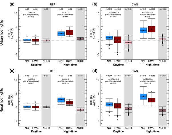
Figure 4. UHII and UHII change (∆UHII) during normal conditions, and (a), (b) urban and (c), (d) rural hot nights. UHII quantification using (a), (c) high-quality reference stations (REFs) and (b), (d) citizen weather stations (CWSs) during daytime (13–16 h UTC + 1) and night-time (01–04 h UTC + 1). See figure 2 for further details.
Download figure:
Standard image High-resolution imageIn contrast, decreased mean night-time UHII can also be found. Such results arise when hot nights are identified at rural locations (figures 4(c) and (d)). REFs and CWSs measure a significant and large effect of decreased mean night-time UHII of −1.02 K and −1.28 K (both p < 0.001), respectively. All REFs show negative night-time ∆UHII during rural hot nights, as well as 1943 out of the 1945 CWSs (=99.9%). Daytime UHIIs preceding rural hot nights show a very small mean effect compared to normal conditions for REFs (not significant), while CWSs again display a significant reduction in mean UHII of −0.57 K (figures 4(c) and (d)).
Generally, weather conditions during rural hot nights and preceding daytime are counterproductive for UHI formation (figure 5, table 1). Though downwelling radiation is significantly higher than during normal conditions, cloud cover fraction, wind speed, and precipitation are increased after midday and significantly higher during night-time (table 1). Such conditions attenuate UHIIs (Morris et al 2001, Kim and Baik 2005, Erell and Williamson 2007, Arnds et al 2017, Beck et al 2018), explaining negative night-time ∆UHII. During nearly one third of rural hot nights precipitation was recorded, compared to only 13.2% of days during normal conditions (table 1). Developing cloud cover during the day, convective precipitation events, and passage of thunderstorms with precipitation have marked diminishing effects onto UHIIs (Gedzelman et al 2003, Fortuniak et al 2006). Besides, atmospheric humidity during rural hot nights is significantly higher than during hot days (compare figures 3(f) and 5(f), table 1), which might also contribute to significantly higher downward longwave radiation during night-time (figure 5(b), table 1) (Sun et al 2017). Moist conditions contribute to decreased UHIIs, as rural locations cool less efficiently than under dry conditions (Scott et al 2018).

Figure 5. Same as figure 3 but for rural hot nights.
Download figure:
Standard image High-resolution imageContradictory results of UHIIs during hot nights are found for Berlin, depending on whether they are defined based on urban or rural night-time T, since the occurrence of these episodes is profoundly different. Less than half of rural hot nights are preceded by a hot day (figure 6(a)), while urban hot nights predominantly follow hot days (70% of the cases, figure 6(b)). This emphasizes that urban populations are much more exposed to conditions that are potentially hazardous than rural dwellers: Urban areas are subject to the hottest night-time conditions following the hottest daytime conditions, hindering recuperation of the human body at night after hot daytime conditions (Laaidi et al 2012). Night-time UHII is strongest during these occasions compared to urban hot days or hot nights alone. For the rural case (figure 6(a)) strongest night-time UHII is found for hot days occurring alone, being similar to UHII during combined urban HWEs (not shown). Combined rural HWEs lead to moderate UHII due to negative mean ∆UHII during rural hot nights (figures 4(c) and (d)).

Figure 6. Occurrences of hot days and hot nights at (a) rural and (b) urban reference locations, and if both hot weather episodes occurred together (hot day followed by hot night). The number of each case (n) is displayed next to the colour bars.
Download figure:
Standard image High-resolution image
3.3. Discussion of the effect of definition of HWEs
Our results highlight that the choice of location to identify HWEs, as well as time of day, can have profound effects concerning ∆UHIIs. Night-time ∆UHII during HWEs identified at daytime is insensitive to the choice of location to identify them. This is consistent across other studies that use daytime or daily maximum T for HWE identification (Fenner et al 2014, Schatz and Kucharik 2015, Li et al 2015, 2016, Sun et al 2017, Zhao et al 2018). However, if night-time or daily minimum temperature is used to identify HWEs (Scott et al 2018), the choice of location to identify HWEs is crucial and contrasting results arise (also found in Scott et al 2018). This effect might also explain why another study found increased UHIIs for two out of three investigated cities in Australia (Rogers et al 2019). For the two cities where night-time UHIIs were increased, heat waves (defined using daily maximum and daily minimum T) were identified at an urban location, while for the third city an airport site at the urban fringe was used (Rogers et al 2019).
Similarly, Fenner et al (2019) showed that in Berlin urban-rural contrasts in heat wave characteristics only arise when heat wave definitions applying daily minimum or daily mean T are investigated. These contrasts could not be found when using heat wave definitions that apply daily maximum T (Fenner et al 2019). Note that given the diverse findings in other studies concerning UHIIs during HWEs, our findings might not be transferable to other regions, as only one mid-latitude city was investigated. However, the impact that methodological differences can have onto results underscores the need for studies such as this one to understand mechanisms behind the observed phenomena. Similar systematic investigations in other cities of different size and located in different climate regions would be of high value in this respect.
3.4. Discussion of possible future UHIIs due to climate change
Since weather conditions have such a strong influence onto UHIIs, the more general question whether UHIIs are exacerbated or reduced under future climate could also be investigated in this respect. Diverse and even contradictory results for the same region or city are reported concerning UHIIs under projected climate change, with most studies showing no or only moderate change in UHIIs (Chapman et al 2017 and references therein). Several studies that investigated projected future UHIIs found that its change, even if small, is often connected to a change in soil moisture (McCarthy et al 2010, Oleson 2012, Hamdi et al 2016). Soil moisture and its link to thermal admittance as well as to the surface energy balance via evapotranspiration/latent heat flux impacts UHIIs (Runnalls and Oke 2000, Chow and Roth 2006, Schatz and Kucharik 2014), also during HWEs (Li et al 2015, Ramamurthy and Bou-Zeid 2017, Zhao et al 2018). Soil moisture is also strongly linked to the occurrence, persistence, and intensity of HWEs (Fischer et al 2007, Hirschi et al 2010, Lorenz et al 2010, Miralles et al 2014). However, as soil moisture is strongly dependent on precipitation, and since different general circulation models (GCMs) show large variability in simulated precipitation on a regional level (Hawkins and Sutton 2011), results concerning UHIIs of regionally downscaled GCM data are strongly influenced by the driving GCM (Grossman-Clarke et al 2017). Studies utilizing an ensemble of GCMs (e.g. Lauwaet et al 2015, Wouters et al 2017) to investigate projected future UHIIs are thus needed for robust results.
In summary, given the strong impact of weather conditions onto UHIIs, in combination with the modest capabilities of GCMs to simulate clouds (IPCC 2013), and the fact that projected changes in soil moisture are not robust in many regions of the world (IPCC 2013), future UHIIs remain uncertain. But even if UHIIs remained unaltered or even decreased in future climate as driven by weather conditions, widespread adaptation measures and reduction in greenhouse gas emissions are needed to counteract the impacts of urbanization and global warming onto local T (Georgescu et al 2013, Sun et al 2016, Wouters et al 2017, Krayenhoff et al 2018). Moreover, adaptation to extreme heat waves is indispensable, since such events have occurred in the past and under present-day climate due to the natural variability of weather and climate (Dole et al 2011).
4. Conclusions
Using an observational data set covering four years in the urban region of Berlin, UHIIs and weather conditions during HWEs were investigated. It was systematically examined how the choice of location and time of day to determine HWEs can lead to contrasting results concerning ∆UHII. The choice of location to identify hot daytime weather is inconsequential for ∆UHII. Contrasting, if HWEs are defined by night-time conditions, the choice of location to identify them has profound impact onto results. While hot urban night-time conditions lead to exacerbated UHIIs, hot rural night-time conditions are associated with reduced UHIIs. Known synoptic drivers of UHII such as cloud cover, wind speed, and precipitation are distinctly different between rural and urban hot nights, thus explaining contrasting ∆UHIIs.
The results suggest that the choice of study design can have a determining influence onto results concerning ΔUHII during HWEs, which also explains some of the contrasting results found in previous studies. This study further highlights the differences of ∆UHIIs between daytime and night-time, as well as a strong dependency on weather conditions, which drive ∆UHIIs during HWEs. Consequently, studies investigating UHIIs during HWEs need to emphasize these aspects. In summary, the results clearly underline that present-day mean UHIIs cannot simply be added to climate change projections to estimate future urban climate conditions (Chapman et al 2017). The question if UHIIs in general and during HWEs might change in the future is strongly linked to the question if and how weather conditions might change (Chapman et al 2017), which will determine future heat-stress hazards in cities.
Acknowledgments
We thank all Netatmo CWS owners in Berlin who shared their data. We further thank Tom Grassmann for support concerning the CWS data, as well as Hartmut Küster and Ingo Suchland for maintaining the weather stations of the Technische Universität Berlin. Jochen Werner is thanked for support concerning the preparation of the meteorological data of the Freie Universität Berlin. DF acknowledges funding by the Deutsche Forschungsgemeinschaft (DFG) as part of the research project 'Heat waves in Berlin, Germany—urban climate modifications' (Grant No. SCHE 750/15-1) (DF). AH and IL received financial support from the German Federal Ministry of Education and Research as part of the research program 'Urban Climate Under Change' [UC]2, contributing to 'Research for Sustainable Development' (FONA), within the research project 'Three-dimensional observation of atmospheric processes in cities (3DO)' (Grant Nos. FKZ 01LP1602 and 01LP1602C, respectively). We acknowledge support by the German Research Foundation and the Open Access Publication Fund of TU Berlin.
Meteorological data from the German Meteorological Service can freely be obtained at the Climate Data Center: https://opendata.dwd.de/climate_environment/CDC/. Elevation data from the Shuttle Radar Topography Mission version 4.1 are freely available at: http://srtm.csi.cgiar.org. Land cover information according to the Global Human Settlement Layer, product 'GHS S-MOD', are provided by the European Commission and freely available at: https://ghslsys.jrc.ec.europa.eu/ghs_smod.php. Netatmo CWS data can freely be obtained via the company's application programming interface at: https://dev.netatmo.com/en-US/dev. All air temperature data from FUB and TUB stations are available upon reasonable request from the authors.
Author contributions
DF initially conceived the study, performed the analyses, and mainly wrote the paper. DF and IL compiled the meteorological data. All authors contributed to the design of the research, continuously discussed the results, and contributed to the writing of the paper.
Competing interests
The authors declare no competing interests.