

Abstract
Ocean primary production (PP), representing the uptake of inorganic carbon through photosynthesis, supports marine life and affects carbon exchange with the atmosphere. It is difficult to ascertain its magnitude, variability, and trends due to our inability to measure it directly at large scales. Yet it is paramount for understanding changes in marine health, fisheries, and the global carbon cycle. Using assimilation of ocean color satellite data into an ocean biogeochemical model, we estimate that global net ocean PP has experienced a small but significant decline −0.8 PgC y−1 (−2.1%) decade−1 (P < 0.05) in the 18-year satellite record from 1998 to 2015. This decline is associated with shallowing surface mixed layer depth (−2.4% decade−1) and decreasing nitrate concentrations (−3.2% decade−1). Relative contributions to PP by various types of ocean phytoplankton have changed, with decreases in production by intermediate-sized phytoplankton represented by chlorophytes (−14.3% decade−1). This is partially compensated by increases from the unique, more nutrient-efficient, coccolithophores (8.4% decade−1). Geographically, the North and Equatorial Indian Oceans are responsible for much of the decline in PP, falling 0.16 and 0.69 PgC y−1 decade−1, respectively. Reduced production by large, fast-growing diatoms along with chlorophytes characterizes the decline here. In contrast, increases in PP are found in the North and North Central Pacific. The increases here are led by chlorophytes in the North Pacific and the small cyanobacteria in the North Central Pacific. These results suggest that the multi-decadal satellite observational record, coupled with an underlying representation of marine biodiversity in a model, can monitor the uptake of carbon by phytoplankton and that changes, although small, are occurring in the global oceans.
Export citation and abstract BibTeX RIS

Original content from this work may be used under the terms of the Creative Commons Attribution 3.0 licence. Any further distribution of this work must maintain attribution to the author(s) and the title of the work, journal citation and DOI.
Introduction
Understanding changes in global ocean primary production (PP) is one of the pressing issues in ocean biogeochemistry. It represents the uptake of carbon via photosynthesis to support growth of phytoplankton at the base of the food web. It is a process that affects the global carbon cycle (Kwiatkowski et al 2017), fisheries (Stock et al 2017), and the state and variability of life in the oceans.
Past, present, and future changes in PP have been the subject of much effort in oceanography. For the past, a 46-year coupled physical-biological model hindcast suggested a decline of 6.5% (Laufkötter et al 2013), which corresponds to −1.4% decade−1. For the future, coupled physical–biological model intercomparison efforts showed disagreement in predicted global ocean PP in a changing climate. Bopp et al (2013) forecast a mean decline of 8.6% by the end of the century (∼1.1% decade−1), similar to Moore et al (2018) who predicted a 24% decline by the year 2300 (∼0.9% decade−1). Laufkötter et al (2015), however reported that 4 of 9 coupled physical-biological models suggested no or positive change. For the present, availability of global ocean color satellite observations can help immensely by providing large-scale, routine observations of chlorophyll, the main pigment of the phytoplankton that are responsible for most ocean PP. Many algorithms have been developed to estimate PP from satellite-derived chlorophyll observations Carr et al (2006).
Although satellite observations are our best source of global phytoplankton chlorophyll, translating these observations into PP is non-trivial. PP is complex, involving cellular physiology, the dynamical physical environment, the ambient irradiance field, and the interactions among them. For example, it is difficult to derive photoadaptation from ocean color satellite observations, which is an important factor for estimating phytoplankton growth and production (Behrenfeld et al 2016). Also phytoplankton growth is responsive to integrated spectral irradiance, rather than bulk estimates of photosynthetically available radiation. Ocean color satellites are nominally global in their ocean coverage, but they are limited by darkness in high latitudes, clouds, aerosols, and sun glint in mid-to-low latitudes, and daily gaps in coverage due to orbital constraints. Finally, satellites do not retrieve information beyond a limited depth and PP is a vertical integral.
Coupled three-dimensional biological-physical models (Buitenhuis et al 2013) are capable of synthesizing these complexities in physiologically mechanistic ways that are consistent with the local environment. Especially important are changes with depth that are explicitly resolved. Also included can be phytoplankton diversity, temperature, nutrient availability, ambient light field, horizontal and vertical mixing (diffusion), advection, carbon-chlorophyll ratios that are dependent on the ambient light field, and inorganic-organic carbon chemical conversions. The disadvantage is that none of these processes and variables in a model is a faithful representation of the natural environment.
By combining the strengths of models with estimates of surface chlorophyll concentrations from satellites, we can potentially improve the representation of global PP. By assimilating the satellite data into models, we can explicitly maximize the strengths of each, while recognizing that the entire complex assortment still holds errors and mischaracterizations. Here we utilize satellite data from the latest NASA processing revisions and assimilate into a model that contains sufficient complexity and heritage to estimate global open ocean (pelagic) PP and trends over the 18-year time series (1998–2015) of the satellite record.
Methods
Satellite mission data sets
Ocean color satellite mission data sets from the Sea-viewing Wide Field-of-view Sensor (SeaWiFS; launched in 1997), Moderate Resolution Imaging Spectroradiometer (MODIS)-Aqua (launched in 2002), and Visible Infrared Imaging Radiometer Suite (VIIRS; launched in 2011) produce global coverage of ocean chlorophyll for the period 1998–2015. The latest version (R2014) substantially reduces inter-mission differences, by virtue of (1) correction for radiometric drift of MODIS-Aqua data (Meister and Franz 2014), and (2) addition of a new chlorophyll algorithm (Hu et al 2012). Some residual biases remain, which are corrected using in situ data (the Empirical Satellite Radiance-In situ Data (ESRID) methodology (Gregg et al 2009)) for chlorophyll values >0.2 mg m−3 and additional regional bias-correction applications for the SeaWiFS mission (Gregg et al 2017) in the northern high latitudes.
Global three-dimensional model and data assimilation
Global ocean biogeochemical dynamics are simulated by the NASA Ocean Biogeochemical Model (NOBM; Gregg et al 2009). Together with a circulation model, Poseidon (Schopf and Loughe 1995), the model has 14 vertical isopycnal layers and spans –84° to 72° latitude at 1.25° longitude by 2/3° latitude spatial resolution. It resolves only open (pelagic) ocean areas, where bottom depth >200 m. It is forced with surface wind stress and longwave radiation, and relaxes to sea surface temperature data, all from the Modern-Era Retrospective analysis for Research and Applications (MERRA). Shortwave radiation forcing is from the Ocean-Atmosphere Spectral Irradiance Model (OASIM, Gregg and Casey 2009).
NOBM contains four phytoplankton groups, diatoms, chlorophytes, cyanobacteria, and coccolithophores, to represent the diversity in the global oceans. Diatoms in the model are high growth, fast sinking, silicate-dependent phytoplankton that have high nutrient requirements. Cyanobacteria are the functional opposite, with slow maximum growth rates, slow sinking, and low nutrient requirements. They additionally have a capability for nitrogen fixation. Coccolithophores are moderate growers that sink relatively quickly due to their calcium carbonate coccoliths. They are efficient users of nitrogen, enabling them to flourish in low nutrient regions (although not as efficient as cyanobacteria). Finally, chlorophytes represent the diverse functionality associated with nanoplankton, with growth rates, sinking rates, and nutrient requirements intermediate between the functional extremes and the more specialized coccolithophores.
Phytoplankton growth is a function of scalar quantum irradiance, which is a measure of the photons impacting phytoplankton cells from all directions, expressed as units of μmol photons m−2 s−1 (Kirk 1992). Variable carbon to chlorophyll ratios are utilized, that depend on the light history and photoadaptation, which is explicit in the model (Gregg and Casey 2007). The model also contains four nutrients (nitrate, ammonium, silicate, and dissolved iron) and three detrital components (particulate organic carbon, silicate, and iron).
PP is computed in the model as a function of growth rate multiplied by the chlorophyll concentration and the carbon: chlorophyll ratio

where μi is the net growth rate (gross growth minus respiration, d−1) of phytoplankton component i as a function of nutrients (N), temperature (T), and quantum irradiance (I), Ci is the chlorophyll concentration of phytoplankton component i, Φ is the carbon:chlorophyll ratio g g−1, and the product is integrated over depth. The term I (quantum irradiance) is the wavelength-integrated irradiance in quanta (mol photons m−2 s−1) available for phytoplankton growth at each model vertical layer. The spectral irradiance at the surface and through the water column are derived using OASIM for the period 1998–2015. This model computes spectral irradiance in 33 bands for the domain 200 nm–4 μm, at the ocean surface as a function of atmospheric optical properties, and then propagates the spectral irradiance downward and upward through the water column as a function of ocean optical properties. OASIM utilizes 25 nm spectral resolution in the visible bands. OASIM spectral irradiance is the source for quantum irradiance in equation (1). MODIS-Aqua and Terra cloud data needed for OASIM are not available for 1998–1999, so climatologies are used for these years. All other atmospheric optical properties are available for the duration of the time series. Only wavelengths between 300 and 700 nm are reported here because of their importance for PP.
NOBM has been a participant in a comparison of global PP algorithms/models (Carr et al 2006). With a global estimate of 38 PgC y−1, NOBM falls in the lower end of intercomparisons. This difference is mostly related to the pelagic nature of the NOBM domain and to the restriction to 72°N latitude. In a different comparison with one of the more popular satellite algorithms (Behrenfeld and Falkowski 1997), NOBM was within about 6 PgC y−1 (NOBM higher) over the same domain (Rousseaux and Gregg 2014). Additionally, a phytoplankton-differentiated satellite algorithm (Uitz et al 2010) was evaluated and produced global PP 7 PgC y−1 higher than NOBM (Rousseaux and Gregg 2014). NOBM has also been a participant in other PP intercomparisons, including the tropical Pacific Ocean (Friedrichs et al 2009) and Bermuda Atlantic Time-Series and Hawaii Ocean Time-Series (Saba et al 2010).
We integrate the model 120 years under climatological atmospheric forcing from MERRA and assimilation of climatological MODIS-Aqua ocean chlorophyll data to obtain stability (defined as near zero trend; Rousseaux and Gregg 2015). Then we run forward from September 1997 until 2015 using transient forcing from MERRA, and ocean color data assimilation, switching from SeaWiFS to MODIS in January 2003 and from MODIS to VIIRS in 2012.
Coupled model/data assimilation/bias correction system and error characterization
There are three main components in this investigation: (1) a global coupled-physical three-dimensional model of the oceans, (2) assimilation of global ocean color data from three different satellite sensors, and (3) adaptation of satellite ocean color data for improved consistency across multiple satellite and in situ data sets. All three have undergone comprehensive error characterization.
- (1)Global coupled-physical three-dimensional model of the oceans. This focuses on the NOBM, the main features of which have been described above. It has been extensively validated against globally distributed in situ data and satellite data when and where available (Gregg and Casey 2007). Three of the four phytoplankton groups exhibited statistically positive correlations with in situ data (P < 0.05) and low bias, as did nitrate, silicate, and dissolved iron. Total chlorophyll was statistically positively correlated with in situ and satellite ocean color data, as well. Chlorophytes were positively correlated but lacked statistical significance due to their model role of representing the large diversity of intermediate phytoplankton in the oceans (Gregg and Casey 2007).Of the 10 model variables relevant to the present work, all but three have been compared with in situ and/or satellite data sets. These three are detritus, ammonium, and herbivores. There are no global detritus, ammonium, or herbivore databases publicly available to our knowledge.The main purpose of NOBM is to provide global, dynamic, depth-resolved biological variables, with complete temporal representation. These aspects are essential for estimating global PP. As a model, NOBM is comprehensive but lacks fidelity with the natural biogeochemical system, despite the statistical comparisons described above. Satellite observations provide more realistic estimates of global chlorophyll concentrations and as such are used to enhance the model results through data assimilation. The constant confrontation with data in the assimilation process steers the model away from its inherent drift tendencies and provides more realistic representations of global chlorophyll.
- (2)Assimilation of global ocean color data from satellite sensors. The capability of data assimilation to improve the representation of global chlorophyll has also been extensively evaluated. A rigorous comparison of chlorophyll from NOBM assimilation of SeaWiFS against independent in situ data over a 6-year time period from 1998 through 2003 indicated a bias in the assimilation model of 0.1% and an uncertainty of 33.4% for daily coincident, co-located data (Gregg 2008). SeaWiFS bias compared with in situ data was slightly higher at −1.3% with nearly identical uncertainty at 32.7%. Model bias and uncertainty without data assimilation were −1.4% and 61.8%, respectively.Assimilation not only corrects the model, it also corrects sampling errors in the satellite data. Ocean color sensors only observe about 15% of the global oceans per day (Gregg et al 1998). Models provide complete daily coverage. The 15% of the oceans observed by satellite occur in the best places and times for phytoplankton growth: the highest solar elevations and the clearest skies. Persistent clouds in some regions obscure many regions to 3 or fewer observations per month. In the high latitudes, whole seasons are missing. This leads to important biases in satellite-based estimates of chlorophyll and PP. These biases are primarily in the direction of overestimation. Our estimates of global ocean chlorophyll using data assimilation are typically about 25% lower than satellites. These biases migrate into satellite-derived PP estimates.
- (3)Adaptation of satellite ocean color data for reduced bias and improved consistency across multiple satellite data sets. Satellite estimates of ocean chlorophyll have their own biases and uncertainties with respect to in situ data. We address this issue using the Empirical Satellite Radiance-In situ Data (ESRID) methodology (Gregg et al 2009). ESRID forces satellite radiances to agree with in situ data, which we take from the five major international in situ data archives (see Acknowledgments). ESRID is substituted for the NASA standard algorithm at chlorophyll concentrations >0.2 mg m−3 (Gregg et al 2017).
VIIRS requires a modification to ESRID because there is insufficient in situ data in the major in situ archives to apply ESRID. Instead we utilize ESRID-MODIS to derive empirical relationships with VIIRS satellite radiances (Gregg et al 2017). Statistics on comparisons with data of ESRID-SeaWiFS and ESRID MODIS with in situ data and ESRIDS-VIIRS show the bias and uncertainty in table 1.
Table 1. Bias and uncertainty (expressed as semi-interquartile range (Gregg et al 2009) as compared with in situ data from major international archives (see Acknowledgments) for ESRID-SeaWiFS, ESRID-MODIS. ESRIDS-VIIRS is compared with ESRID-MODIS.
| Ocean color sensor | Bias | Uncertainty | Correlation |
|---|---|---|---|
| SeaWiFS | 15.8% | 35.7% | 0.870 |
| ESRID-SeaWiFS | −5.1% | 34.4% | 0.868 |
| MODIS-Aqua | 17.2% | 32.2% | 0.854 |
| ESRID-MODIS | −3.7% | 32.3% | 0.863 |
| VIIRS | 11.8% | 27.9% | 0.857 |
| ESRIDS-VIIRS | 1.4% | 26.9% | 0.864 |
The three approaches used here: global coupled physical-biological dynamical model to resolve vertical resolution necessary for estimating PP and to provide complete daily representation of the global oceans, data assimilation to correct the model for biases, and in situ data to correct satellite data for their individual biases, produce a unique perspective to evaluate global PP trends in the modern ocean color record. Together they provide a global representation of PP with attention to minimizing the biases, uncertainties, and sampling issues inherent in each.
Statistical treatment of PP trends
We derive trends using linear regression analysis on global annual net PP from satellite data assimilation and associated biological variables by (1) integrating annual PP spatially at each model grid point by depth and day, (2) aggregating data over ocean basins and globally, (3) correcting for end-point bias (Gregg and Rousseaux 2014), (4) deriving best fit linear trends, and (5) evaluating statistical significance of the trends. A statistically significant trend exceeds the 95% confidence level.
End-point bias correction is applied to prevent anomalous data at the beginning or end of a time series from overly influencing the detection of a trend. In the case of our 18-year time series, both the beginning (1998) and end years (2015) are associated with unusually strong El Niño events. This is an unfortunate artifact of the launch of the first modern ocean color sensor, and the end which marks the completion of a verified processing version. The 1998 El Niño caused few issues in the time series trends, because higher surface ocean temperatures succeeded it, and thus it is not the highest in the series. The 2015 event, since it occurred at the end of the series and represented the highest surface temperature observed in the series, produced maxima or minima of several of the reported variables in this analysis. Reporting a trend when in fact it is an artifact of an unusual event occurring at the beginning or end, and when it produces a significant trend that otherwise would not exist, is a classic manifestation of end-point bias. Observation of a trend in these circumstances, increases the probability of a Type-1 error, i.e. finding a significant trend where one does not exist (Zar 1976). We remove the end point in these cases and report lack of significance in the trend. This occurs for surface temperature, diatoms, and cyanobacteria for global time series.
Although it is established that global sea surface temperature has increased over the past several decades (Hausfather et al 2017, Huang et al 2017, Lian et al 2018), our analysis shows no significant trend (after end-point bias correction). This is because our observational period 1998–2015, which is defined by the availability of modern ocean color satellite data and established data processing, unfortunately falls in a period bracketed by two major ENSO events, as mentioned above. For 2000–2015 we find a significant positive trend of 0.108° decade−1, which is similar to the trend reported by Huang et al (2017), 0.125° decade−1 for the Extended Reconstructed Sea Surface Temperature, Version 5.
The trends reported here are not corrected for autocorrelation. The ultimate purpose of autocorrelation evaluation is to understand the probability of a Type-1 error. Our use of annual data reduces the possibility of Type-1 errors by low sample size and thus degrees of freedom (df), which is df = 16 for the 18-year time series. End-point bias correction further reduces the risk. Additional use of autocorrelation noise correction in annual data with end-point bias correction increases the probability of Type-2 error, i.e. not observing a trend where one exists.
Results and discussion
Global ocean PP shows a small (−0.8 PgC y−1 decade−1) but statistically significant decline (r = −0.648, P < 0.05) in the 18-year time series from 1998 to 2015 (figure 1; table 2). The trend represents a reduction of 2.1% decade−1 and suggests a weakening of the biological pump. This is about twice the decline estimated using free-run (not assimilated) models for the future (Bopp et al 2013). Chlorophyte global PP also declines −14.3% decade−1 (r = −0.849, P < 0.05), and is the main contributor to the global trend. Coccolithophores, conversely, increase their PP (8.4% decade−1, r = 0.522, P < 0.05; table 1) over the time series. Production by the functional extreme phytoplankton, diatoms and cyanobacteria, exhibit no significant change. The global total PP decline is associated with a shallowing of the surface mixed layer of 1.4 m decade−1, or 2.4% decade−1 (r = −0.719, P < 0.05; figure 2; table 2). Shallowing mixed layers tend to reduce the supply of nutrients to the surface from the deep ocean, and inhibit PP on annual scales. As a consequence, nitrate, one of the most important nutrients for phytoplankton growth and production, declines 0.18 μM decade−1 (3.2% decade−1; r = −0.503, P < 0.05; table 2).
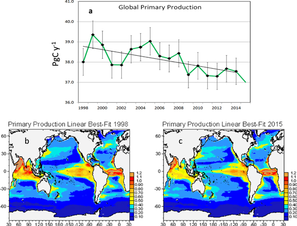
Figure 1. (a) Global primary production trend for 1998–2015. The missing marker for 2015 indicates removal of this value from the trend analysis due to end-point bias correction. Error bars represent the standard deviation. Linear best-fit primary production trends are shown for (b) 1998 and (c) 2015.
Download figure:
Standard image High-resolution imageTable 2. Statistics on trends in global ocean primary production and related variables. NS indicates not significant at 95% confidence level. Trends for variables that are not significant are not shown. The 18-year time series has N = 18, except when end-point bias is observed.
| Global variable | Correlation coefficient | N | Trend |
|---|---|---|---|
| Total primary production | −0.648 P < 0.05 | N = 17 | −0.81 PgC y−1 decade−1 |
| (2.1% decade−1) | |||
| Diatom production | −0.472 NS | N = 17 | |
| Chlorophyte production | −0.849 P < 0.05 | N = 18 | −0.98 PgC y−1 decade−1 |
| (14.3% decade−1) | |||
| Cyanobacteria production | 0.377 NS | N = 17 | |
| Coccolithophore production | 0.522 P < 0.05 | N = 17 | 0.60 PgC y−1 decade−1 |
| (8.4% decade−1) | |||
| Nitrate | −0.503 P < 0.05 | N = 17 | −0.18 μM dec−1 (3.2% dec−1) |
| Ammonium | 0.164 NS | N = 18 | |
| Silicate | −0.408 NS | N = 18 | |
| Chlorophyll | 0.234 NS | N = 18 | |
| Mixed layer depth | −0.719 P < 0.05 | N = 18 | −1.43 m decade−1 |
| (2.4% decade−1) | |||
| Surface temperature | 0.344 NS | N = 17 |
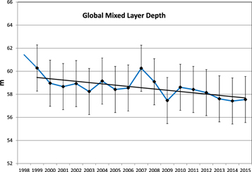
Figure 2. Global mixed layer depth trend for 1998–2015. The missing marker for 1998 indicates removal of this value from the trend analysis due to end-point bias correction. Error bars represent the standard deviation.
Download figure:
Standard image High-resolution imageThese results suggest a consistent representation of recent trends in global ocean PP: shallowing mixed layer restricting nutrient supply produces declining total PP. The global production trend is small, however, and limited to chlorophytes, which have intermediate requirements for nutrients. Their reduction in PP is partially compensated by increasing coccolithophore production. Coccolithophores are more efficient users of nutrients and thus have a competitive advantage in a lower nutrient environment. The changes in phytoplankton contributions are not enough to produce a community shift in contributions to PP.
The global trends do not appear to be related to the El Niño-Southern Oscillation (ENSO) events that have occurred in the time series. There is no significant trend in the Equatorial Pacific and the global trend is statistically similar even if we begin the series as late as 2006.
Using the first global ocean color sensor, Coastal Zone Color Scanner (CZCS) for 1978–1986 and the Sea-viewing Wide Field-of-view Sensor (SeaWiFS) for the period 1997–2002, a 6% decline in global PP was found (Gregg et al 2003). Both data sets were blended with in situ data to remove biases and inconsistencies between them. In that effort, a satellite chlorophyll algorithm (Behrenfeld and Falkowski 1997) was utilized. Assuming that the CZCS record and the partial SeaWiFS record constitute a time span of approximately 20 years, this suggests a decline of about 3% decade−1. This is similar to the 2.1% decade−1 reported here, tentatively suggesting consistency in the nearly 40 years of global ocean color observations.
The North and Equatorial Indian Ocean basins (northward of 10°S) are major contributors to the observed global decline (figure 3). Here regional total production falls −0.16 PgC y−1 (9.7%) decade−1 and −0.69 PgC y−1 (16.2%) decade−1, respectively, over the 18-year time series. The change is most clearly observed in the Bay of Bengal (eastern) portion of the North Indian basin, as well as the eastern portion of the Arabian Sea (figure 3). In the Equatorial Indian there is an overall decline throughout the basin rather than the more localized trends in the North Indian (figure 3).
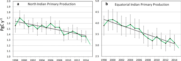
Figure 3. Primary production linear trends are shown for (a) North Indian Ocean and (b) Equatorial Indian Ocean.
Download figure:
Standard image High-resolution imageIn both basins the decline is driven by diatom and chlorophyte PP. Diatom production declines by an average of 15.4% decade−1 for the 2 basins while chlorophyte production declines by 24.8% decade−1 (data not shown). In the Equatorial Indian, the reduction in phytoplankton PP is partially compensated by increases in production by the smaller, more nutrient-efficient, cyanobacteria and coccolithophores. Here, cyanobacteria production increases 16.7% decade−1 in the record while coccolithophore contributions increase nearly ten-fold. This results in a shift in relative contributions to total PP in the basin (figure 4) and is consistent with the more efficient nutrient utilization capabilities of the smaller phytoplankton, the cyanobacteria and coccolithophores.
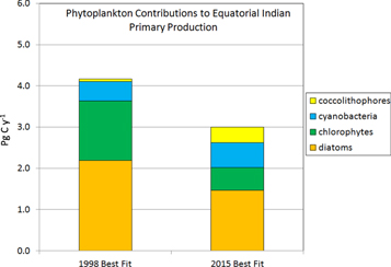
Figure 4. Changes in phytoplankton contributions to total primary production in the Equatorial Indian Ocean 1998–2015. Start and end years are from best-fit linear trends, not the actual years.
Download figure:
Standard image High-resolution imageBoth Indian Ocean basins experience declines in nitrate and silicate (32.4% and 22.8% decade−1, respectively). Silicate is critical for diatom growth and its decline is likely an important cause for their decline. Nitrate is needed by all phytoplankton, which suggests a cause for the reduction in chlorophyte production. At the same time, the smaller cyanobacteria and coccolithophores increase production due to their higher ability to harvest nutrients at lower concentrations, but not enough to overcome a basin-wide decline in total PP. The PP declines are not associated with statistically significant changes of mixed layer depth The Equatorial Indian basin, but not the North Indian, also exhibits increasing surface temperature (0.22° decade−1, r = 0.552).
Strong declines in chlorophyll have been reported in the sub-tropical Indian Ocean over the past six decades (Roxy et al 2016), which suggested associated declines in PP. The results here support this and further document nutrient declines. There is also evidence of sea level rise and associated weakening of the summer monsoon in the Equatorial Indian Ocean in recent decades (Swapna et al 2017). Such weakening could reduce the upwelling of nutrients and suppress ocean PP as we find here.
A modeling effort by Kvale et al (2019) suggested increases of calcifier production in low latitudes under a warming ocean scenario. This was attributed, as here specifically for the calcifying phytoplankton coccolithophores, to their increased ability to utilize nutrients under low availability. Cyanobacteria, which have even more efficient nutrient uptake capabilities, also increase under these conditions of low nutrients, but not as much as coccolithophores. The increases of these smaller phytoplankton comes at the expense of larger phytoplankton, like diatoms, which is also supported by Kvale et al (2019).
In contrast to the global and Indian Ocean trends, total PP in the North and North Central Pacific basins increase over the 18-year time series (figure 5). The increases are 0.05 (4.8%) and 0.2 (4.4%) PgC y−1 decade−1, respectively. The changes in phytoplankton production in the two basins are different: the North Pacific increase is led by chlorophytes PP and the North Central Pacific is led by cyanobacteria production. Chlorophyte production nearly triples in the North Pacific, although it still contributes only 13% of the total, which is dominated by diatom production. In the North Central Pacific, cyanobacteria production increases 6.4% decade−1. Cyanobacteria predominate in abundance in this basin but their PP is next to last (chlorophyte production is lowest). Both basins exhibit shallowing mixed layer depths (9.5% decade−1 in the North Pacific and 6.8% decade−1 in the North Central Pacific). The North Pacific also shows an increase in surface layer temperature (0.4° decade−1, data not shown) while temperature in the North Central Pacific does not significantly change. A summary of the results described here is provided in figure 6.

Figure 5. Primary production trends in the (a) North and (b) North Central Pacific Oceans. The dashed line divides the two at 40oN latitude (note scale change from figure 1). Linear trends for (c) North Pacific Ocean and (d) North Central Pacific.
Download figure:
Standard image High-resolution image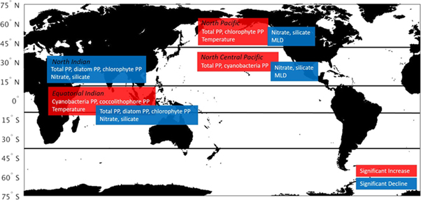
Figure 6. Geographical summary where total primary production showed significant trends For the period 1998–2015 along with associated trends from related physical and biological variables.
Download figure:
Standard image High-resolution image
The combination of a dynamical global biogeochemical model assimilated with bias-corrected ocean color satellite data provides enhanced realism in the representation of recent trends in global ocean PP. However, the results are not unequivocal. Assessment of changes in past, present, and future global PP remains challenging. The time series of global ocean color satellites is still too short to unequivocally distinguish natural variability from long-term trends (Henson et al 2016), but this report provides a marker for the observed intermediate-term trends in the record so far. As state-of-the-art methodologies improve, as knowledge advances, and as the time series continues with new missions, the effort here can stand as a baseline against which future observations can provide perspective.
Acknowledgments
We thank the NASA Ocean Color Processing Team for satellite data sets. This work was supported by NASA S-NPP, PACE, EXPORTS, and MAP Programs. The authors and their affiliations have no real or perceived financial conflicts of interests. The authors have no competing interests. We thank the SeaWiFS Bio-Optical Archive and Storage System, National Oceanographic Data Center, Atlantic Meridional Transect, Hawaii Ocean Time Series, and Biological and Chemical Oceanography Data Management Office for in situ data. Assimilated data for the period 1998–2015 are available at the NASA Giovanni web site.