

Abstract
Reducing emissions from deforestation and forest degradation, and enhancing carbon stocks (REDD+) is a crucial component of global climate change mitigation. Remote sensing can provide continuous and spatially explicit above-ground biomass (AGB) estimates, which can be valuable for the quantification of carbon stocks and emission factors (EFs). Unfortunately, there is little information on the fate of the land following tropical deforestation and of the associated carbon stock. This study quantified post-deforestation land use across the tropics for the period 1990–2000. This dataset was then combined with a pan-tropical AGB map at 30 m resolution to refine EFs from forest conversion by matching deforestation areas with their carbon stock before and after clearing and to assess spatial dynamics of EFs by follow-up land use. In Latin America, pasture was the most common follow-up land use (72%), with large-scale cropland (11%) a distant second. In Africa deforestation was often followed by small-scale cropping (61%) with a smaller role for pasture (15%). In Asia, small-scale cropland was the dominant agricultural follow-up land use (35%), closely followed by tree crops (28%). Deforestation often occurred in forests with lower than average carbon stocks. EFs showed high spatial variation within eco-zones and countries. While our EFs are only representative for the studied time period, our results show that EFs are mainly determined by the initial forest carbon stock. The estimates of the fraction of carbon lost were less dependent on initial forest biomass, which offers opportunities for REDD+ countries to use these fractions in combination with recent good quality national forest biomass maps or inventory data to quantify emissions from specific forest conversions. Our study highlights that the co-location of data on forest loss, biomass and fate of the land provides more insight into the spatial dynamics of land-use change and can help in attributing carbon emissions to human activities.
Export citation and abstract BibTeX RIS

Original content from this work may be used under the terms of the Creative Commons Attribution 3.0 licence. Any further distribution of this work must maintain attribution to the author(s) and the title of the work, journal citation and DOI.
1. Introduction
Land-use change, mainly deforestation, is the second largest source of anthropogenic CO2 emissions, with the majority of this occurring in tropical regions (IPCC 2013). Reducing emissions from tropical deforestation is therefore a crucial component of global climate change mitigation. Within the 'Reducing emissions from deforestation and forest degradation, and enhancing carbon stocks' (REDD+) framework, participating countries are encouraged to develop national strategies and implementation plans that reduce emissions and enhance forest sinks. Systematically measuring, reporting and verifying forest carbon emissions and removals is a key component in the REDD+ framework. Carbon emissions from deforestation can be estimated by combining activity data (AD) with emission factors (EF). AD here refers to the change in forest area, while EF refer to the changes in carbon stock per unit area, e.g. tons carbon emitted per hectare of deforestation.
Carbon stock or flow information on the forest carbon pools can be obtained at three Tiers according to the IPCC guidelines (IPCC 2006). Tier 1 uses global default values (i.e. per ecological zone) derived from the literature, while Tier 2 uses country-specific carbon stock or flow data. In Tier 3 more disaggregated data of carbon stocks in different pools are available from national inventories, through repeated measurements and supported by modelling. In most cases for the 3 Tier levels the emission factors are estimated at a single date corresponding to the data referred in bibliographic reference or to the national inventory. Spatially explicit data on carbon stock is valuable due to the large variation in forest biomass relating to environmental (rainfall, elevation, soil type etc) and anthropogenic (management practices, land use history etc) factors (Gibbs et al 2007). Country or region specific carbon stock data are traditionally derived from forest inventories, which are valuable but often limited in geographic representativeness (Gibbs et al 2007). For AD, tracking land use conversions over time is desirable because human activities (i.e. drivers) can be attributed to forest area change, which can be useful for REDD+ policy making and implementation (De Sy et al 2015). This is preferably done in a spatially explicit manner, in light of the spatio-temporal dynamics of drivers of forest area change (De Sy et al 2015). Remote sensing is considered essential for monitoring forest and other land-use changes (Herold and Johns 2007, De Sy et al 2012).
Capacities of REDD+ countries for forest area change monitoring on the national level have improved (Romijn et al 2015), and a number of REDD+ countries have developed operational sub-national monitoring systems (e.g. for Brazilian Amazon). However, in many REDD+ countries forest inventories are of insufficient quality, geographically limited, and progress is slow (Romijn et al 2015), which means that many countries rely on IPCC Tier 1 default values or simplified assumptions until they build sufficient inventory capacity. Deforestation can occur in forests with lower or higher than average carbon stocks (Baccini et al 2012), which is often not accounted for in Tier 1 or Tier 2 default values. Remote sensing can provide continuous and spatially explicit above-ground biomass (AGB) estimates, which can be valuable for the analysis and quantification of carbon stocks and emission factors (Goetz et al 2009, Saatchi et al 2011, Baccini et al 2012).
Several large scale studies have estimated carbon emissions from tropical deforestation for the 1990s and 2000s, using spatially explicit AD and EF data (DeFries et al 2002, Baccini et al 2012, Harris et al 2012, Achard et al 2014, Grace et al 2014, De Sy et al 2015, Tyukavina et al 2015, Zarin et al 2016). All of these studies, however, base their estimates of carbon emission on lost forest carbon stock only, and do not consider the carbon stock of the land use following deforestation. The fate of the land, and associated carbon stock, will influence the total carbon losses from deforestation. For example, it is generally assumed that mechanised clearing for large-scale agriculture results in a more complete removal of biomass than for smallholder farming and pastures (Houghton 2012). Unfortunately, there is little spatially explicit information on the fate of the land following tropical deforestation (De Sy et al 2015), and of the associated carbon stock. Integrating information on the spatial distribution of deforestation and forest carbon stock density into emission factors will provide more insight into the complex spatial dynamics of tropical forest carbon loss and will allow further refinement of carbon emission estimates for REDD+ country reporting. In addition, integrating information on land use following deforestation, and its carbon stock, adds further refinement and can help in attributing forest loss and carbon emissions to human activities. This will be a valuable source of information for REDD+ monitoring, reporting and strategy development.
Recently, new remote sensing data has become available that can help to address this issue. De Sy et al (2015) quantified land use following deforestation (fate of the land) in South America for the periods 1990–2000 and 2000–2005, with a methodology that can be extended to other tropical areas. Zarin et al (2016) extended the methodology of Baccini et al (2012) to generate a pan-tropical map of above-ground live woody biomass density at 30 m resolution for circa the year 2000. These new datasets allow for the co-location of forest loss, post-deforestation land use and biomass estimates at similar spatial resolutions for the period 1990–2000. This provides an opportunity to refine emission factors (i.e. carbon loss per unit area) from forest conversion by matching deforestation areas with their carbon stock before and after clearing, and to assess spatial dynamics of emission factors by taking into account the follow-up land use.
Accordingly, our study aims to:
- i.Quantify tropical deforestation drivers in Africa, Asia and Latin America.
- ii.Produce carbon stock estimates of tropical forests and land uses following deforestation by country and eco-zone, and derive estimates of emission factors from forest conversion.
- iii.Assess spatial dynamics of emission factors by follow up land use type.
Finally, our study allows making recommendations to improve carbon emission factors as input for REDD+ forest monitoring.
2. Material and methods
Figure 1 gives an overview of the workflow and datasets used in our methodology. We used a systematic sampling approach. In section 2.1 we describe the sampling approach and the methodology for determining deforestation areas and follow-up land use per sample unit (figure 1(A)). In section 2.2 we describe how we arrive at emission factors (EF) per follow-up land use in each sample unit (figure 1(B)). Last, in section 2.3 we describe the method to aggregate these results to the regional level.

Figure 1. Conceptual framework of the methodological steps and datasets.
Download figure:
Standard image High-resolution image2.1. Deforestation and land use following deforestation per sample unit
The Remote Sensing Survey of the Global Forest Resources Assessment 2010 of FAO (FAO FRA-2010 RSS) (FAO and JRC 2012) was used as input to identify deforestation areas. FAO FRA-2010 RSS is a spatially explicit dataset of forest land-use change from 1990 to 2000 and 2000 to 2005 (figure 1(A)). The FAO FRA-2010 RSS used a systematic sampling design with sample units (SU) of 10 by 10 km centred on each degree latitude–longitude intersection point (Eva et al 2012, FAO and JRC 2012, Achard et al 2014). This leads to a sample of 4000 SUs over the tropics. Each SU was segmented into delineated areas (polygons) with a target minimum mapping area of 5 ha. Then, a supervised automated land cover classification was carried out. This was later converted to a land use classification with the help of expert human interpretation. Figure 2 gives an overview of our study area, all sample units and the FAO ecological zones (eco-zones) (FAO 2001) in our study area.

Figure 2. Location of sample units (FAO and JRC 2012), and ecological zones (FAO 2001) in the study area.
Download figure:
Standard image High-resolution imageAs the land use classification of the original FAO FRA-2010 RSS study was limited, we assigned a more detailed (follow-up) land use classification for each forest loss area by extending the methodology of De Sy et al (2015) for South America to a larger study area (Latin America, Africa, part of Asia). De Sy et al (2015) identified spatial and temporal land use patterns following tropical deforestation in South America for 1990–2005. For this study, we only assigned follow-up land use to deforested areas in the time period 1990–2000 (figure 1(A)), as this corresponds best with the pan-tropical map of above-ground live woody biomass density (hereafter referred to as AGB map).
We classified the follow-up land use by visual interpretation, using parameters such as land cover, the presence of certain features within or near changed areas (e.g. crop rows, watering holes, fences) and the spatial context and location of change (e.g. distance to settlements, concessions). Table 1 gives an overview of the follow-up land use classes and their descriptions. A variety of satellite imagery was used for the visual interpretation such as Landsat, Google Earth imagery (Google Earth 2017) and ESRI world imagery base maps. In addition to follow-up land use, the confidence (low–medium–high) in the interpretation was documented. For areas with low confidence, e.g. due to low resolution imagery, we consulted land use and remote sensing experts with local knowledge in order to classify the areas based on their expert knowledge, and on additional sources available to them such as high resolution satellite imagery and land use maps. Finally, all areas were double checked for errors and consistency. This means each forest loss area has been checked at least twice by one or more experts. De Sy et al (2015) provides more details on the follow-up land use classification methodology.
Table 1. Follow-up land uses and their description.
| Follow-up land use | Description | |
|---|---|---|
| Agriculture | Mixed agriculture | Mix of agricultural land uses |
| Large-scale crop | Land under cultivation for crops, characterized by medium (2–20 ha) to large (>20 ha) field sizes | |
| Small-scale crop | Land under cultivation for crops, characterized by very small (<0.5 ha) to small field sizes (0.5–2 ha) | |
| Tree crops | Miscellaneous tree crops (e.g. coffee, palm trees), orchards and groves | |
| Pasture | Land used predominantly for grazing; in either managed/cultivated (pastures) or natural (grazing land) setting; includes grazed woodlands | |
| Infrastructure |
|
|
|
||
|
||
| Other land use | All land that is not classified as forest, agriculture, infrastructure and water: | |
|
||
|
||
|
||
|
||
| Water | Natural (river, lake etc) or man-made waterbodies (e.g. reservoirs) | |
| Unknown land use | All land that cannot be classified (e.g. due to low resolution imagery) | |
2.2. Emission factors per sample unit
The emission factor per follow-up land use for each sample unit was calculated from forest carbon stock before deforestation (CForest), and the carbon stock of the land use following deforestation (CFLU). We only considered the five main follow-up land uses with sufficient data for calculating CForest: pasture, large-scale cropland, small-scale cropland, tree crop, and other land use (table 1). We excluded tree crops from the calculation of CFLU and EF as we did not have information on the age of the tree crops.
A pan-tropical 30 m resolution AGB map (Zarin et al 2016) was used to derive the mean AGB density for forest and follow-up land uses for each sample unit (figure 1(B)). This wall-to-wall AGB map represents AGB density for the year c. 2000. We first processed the AGB map to remove as much bias as possible when compared to an extended forest biomass plot database, following the methodology described in Avitabile et al (2016). See the supporting information for a full description of the bias adjustment (S1) is available online at stacks.iop.org/ERL/14/094022/mmedia. We will further refer to the bias adjusted AGB map as the AGB map.
Our deforestation data represent areas deforested before 2000, so we can directly estimate the mean AGB of the follow-up land use per sample unit. Since forest loss occurred between 1990 and 2000 and the AGB map is dated c. 2000, we cannot directly estimate the AGB of the cleared forest. Instead we used the mean AGB of the remaining stable forest (i.e. forest from 1990 to 2005) within a sample unit as a proxy for the AGB of the cleared forest. We assume that within a sample unit the AGB of this stable forest is representative of the cleared forest. So a patch of forest cleared by pasture would get the same AGB for cleared forest as a patch cleared for crop within this sample unit. If no stable forest remained in the sample unit we used an inverse distance weighted average from the 8 surrounding sample units.
In addition, we used the Hansen forest cover dataset (Hansen et al 2013), which has the same resolution (30 m) as the AGB map, as a forest mask for the year 2000 (figure 1(B)) with forest defined as more than 10% tree cover. Although the FAO FRA-2010 RSS provides a forest–non-forest classification, with forest defined as land spanning more than 0.5 hectares and a canopy cover of more than 10% (FAO 2010), a minimum mapping unit of 5 ha was used. Within the 5 ha mapping unit, dominant forest patches might be mixed with small patches of other land uses and vice versa, which results in relatively higher AGB values for follow-up land use polygons and relatively lower AGB values for forest polygons. In addition, since both datasets are from circa 2000, they might not exactly match temporally (e.g. the FRA-2010 RSS dataset targets imagery around 1st July 2000 but depending on data availability imagery is spread along the period 1999–2002, see Beuchle et al 2011). Use of the Hansen tree cover map corrected for this and for spatial inaccuracies between the FAO FRA-2010 RSS and AGB map, by masking out forest pixels in the follow-up land use polygons and non-forest pixels in stable forest polygons.
We derived total biomass from AGB for both follow-up land use and stable forest per sample unit by applying the equation (1) used by Saatchi et al (2011):

In this equation belowground biomass (BGB) is calculated from AGB using a universal equation derived from a synthesis of regression equations developed from field data across multiple biomes (Saatchi et al 2011).
Total carbon was considered to be 50% of total biomass as in Achard et al (2014). We did not account for soil carbon loss.
Finally we derived the emission factor per follow-up land use (EF) per sample unit by:

We also calculated the percentage of carbon lost (EF%):

2.3. Scaling to regional level
Forest area loss, forest carbon stock (CForest), carbon stock of the land use following deforestation (CFLU) and emission factors per follow-up land use were scaled to the national, eco-zone (FAO 2001) and continental levels.
To scale up forest area loss per follow-up land use to the regional (i.e. national, eco-zone, continental) scales, the forest area loss within each sample unit is made proportional to the 'visible land' area of the sample unit. The 'visible land' area was the full sample unit area (100 km2) minus cloudy and 'permanent water' areas (i.e. sea in all considered years). In addition, each sample unit was assigned a weight (wi) (4), equal to the cosine of its latitude (coslati), because the actual area represented by a latitude/longitude grid sample decreased with latitude due to the curvature of Earth:

The proportions of forest area change per follow-up land use in each sample unit were then extrapolated to a given region using the Horvitz–Thompson direct estimator (Särndal et al 1992) (5)

where

and where xic is the proportion of forest area change in the ith sample unit and wi is the weight of the ith sample unit. The total area of forest area change per follow-up land use for this region (FLUregion) is then obtained from:

where A is the total area of the region (excluding permanent water).
The variance of the estimation of the mean for this systematic sample was calculated as follows:

The standard error (SE) is then calculated as:

The standard error (SE) represents only the sampling error.
For scaling up the mean carbon stocks of the land uses following deforestation (CFLU) and emission factors per follow-up land use (EF) to regional level, we calculated a weighted mean of all sample unit values within that specific region. The weight was determined using wi (4) and 'visible land area' (i.e. sample unit area minus cloudy and 'permanent water' areas) as above. We derived the regional values of carbon stock of forest cleared by a given land use (e.g. pasture) from weighted averaging all the carbon stocks of stable forests in sample units where forests were cleared by this given land use (e.g. pasture). The regional values of carbon stock of 'All forests' comes from averaging all carbon stock values of stable forest for all sample units with forests (whether these were deforested or not). If there were less than five sample units for a follow-up land use in a region, the results are not shown. If there were less than ten sample units present, an annotation was added. We performed a permutation test with 1000 iterations to assess if (1) mean carbon stock of follow-up land uses and (2) mean carbon stocks of all forests, all converted forests and forests converted to a specific land use were significantly different (p < 0.05) within a region.
3. Results
3.1. Deforestation per follow-up land use from 1990 to 2000
We estimated that the total deforested area from 1990 to 2000 was 40.5 million hectares for the Latin American study area, 19.7 million hectares for the African study area and 16.6 million hectares for the Asian study area (table 2). In all regions agriculture is the dominant follow-up land use. In the Latin American countries, deforestation is followed by pasture (72.2%) and to a lesser extent by large-scale cropland (10.9%). In Africa deforestation is more often followed by small-scale cropland (61.1%), with a smaller role for pasture (14.7%). In the Asian study area, small-scale cropland is also the most dominant agricultural follow-up land use (35.0%), closely followed by tree crops (27.9%). In the non-agricultural category, other land use was important in the Asian region (30.1%). Other land use was less important in the African (15.5%) and Latin American regions (6.8%). Infrastructure accounted for 3.3% of deforestation in the Asian region, and for only 1.8% and 1.3% respectively in the Latin American and African study area. More detailed information on the spatial distribution of follow-up land uses across the study area can be found in the supporting information (S2).
Table 2. Estimates of deforested area (103 ha (SE) and % of total) per follow-up land use (table 1) from 1990 to 2000.
| Africa | Latin America | Asia | ||||
|---|---|---|---|---|---|---|
| Follow-up land use | 103 ha | % | 103 ha | % | 103 ha | % |
| Small-scale crop | 12 028 (1174) | 61.1 | 1419 (269) | 3.5 | 5813 (921) | 35.0 |
| Large-scale crop | 812 (425) | 4.1 | 4429 (864) | 10.9 | 89 (36) | 0.5 |
| Tree crop | 476 (194) | 2.4 | 253 (63) | 0.6 | 4630 (1078) | 27.9 |
| Pasture | 2883 (811) | 14.7 | 29 272 (2259) | 72.2 | 210 (66) | 1.3 |
| Mixed agriculture | 35 (30) | 0.2 | 372 (264) | 0.9 | 91 (59) | 0.5 |
| Total agriculture | 16 234 (1552) | 82.5 | 35 745 (2456) | 88.2 | 10 832 (1441) | 65.2 |
| Infrastructure | 255 (41) | 1.3 | 735 (264) | 1.8 | 554 (119) | 3.3 |
| Other land use | 3050 (419) | 15.5 | 2760 (363) | 6.8 | 5000 (1076) | 30.1 |
| Water | 72 (29) | 0.4 | 1220 (476) | 3.0 | 206 (57) | 1.2 |
| Unknown | 69 (51) | 0.3 | 88 (77) | 0.2 | 29 (28) | 0.2 |
| Total other | 3446 (429) | 17.5 | 4803 (719) | 11.8 | 5789 (1128) | 34.8 |
| Total | 19 679 (1663) | 100 | 40 548 (2613) | 100 | 16 621 (1916) | 100 |
3.2. Carbon stocks and emission factors per follow-up land use
Table 3 presents the mean carbon stock (Mg C ha−1) of all forests within an eco-zone, and the mean carbon stock of forests that were cleared and followed by pasture, large-scale cropland, small-scale cropland, other land use, and tree crop.
Table 3. Mean carbon stock estimates (Mg C ha−1) for all forests, for forests converted to any of the follow-up land uses and for forests converted to a specific follow-up land use (pasture, large-scale cropland, small-scale cropland, other land use or tree crop), aggregated to continental and eco-zone levels. Values are mean (standard error). Any two means sharing the same letters within a region are not significantly different (p < 0.05) according to a Permutation Test with 1000 iterations. For example, for the tropical rainforest zone in Africa, the mean carbon stock estimate of 'Forests converted to Tree crop' is significantly different from the mean carbon stock estimate of 'All forests' (do not share same letter), but is not significantly different from the mean carbon stock estimate of 'Forests converted to Small-scale cropland' (share same letter).
| Forests converted to | ||||||||
|---|---|---|---|---|---|---|---|---|
| Region | All Forests | Forests converted to any follow-up land use | Pasture | Large-scale cropland | Small-scale cropland | Other land use | Tree crop | |
| Continent | Africa | 76 (86)a | 41 (60)a | 10 (7) | 10 (6)a | 53 (69) a | 19 (24) a | 72 (58) a |
| L. America | 128 (58) | 85 (43) ad | 86 (44) ab | 77 (25)c | 103 (59) d | 85 (39) ad | 54 (28) bc | |
| Asia | 156 (70) a | 128 (60)ad | 89 (27)b | 100 (21) bcd | 122 (61) cd | 125 (62) a | 139 (58) c | |
| Tropical rainforest | Africa | 155 (81) a | 96 (87) a | — | — | 107 (91) ab | 77 (78)* ab | 78 (59) b |
| L. America | 155 (44) | 111 (39) a | 114 (37) a | 88 (31) b | 117 (62) a | 109 (37) a | 54 (34) b | |
| Asia | 174 (68) a | 131 (62) ac | 94 (27)* ab | — | 123 (63) bc | 125 (64) ac | 144 (59) b | |
| Tropical moist deciduous forest | Africa | 24 (18) a | 17 (11) a | 10 (8) a | 9 (8)* a | 19 (11) a | 17 (8) a | 18 (4)* a |
| L. America | 76 (50) ab | 59 (22) c | 56 (20) c | 72 (20) ac | 75 (43) abc | 65 (22) ac | 47 (14) b | |
| Asia | 100 (31) a | 95 (21) a | 83 (31)* a | 101 (11)* a | 96 (20) a | 95 (25) a | 91 (18) a | |
| Tropical dry forest | Africa | 13 (14) ab | 13 (11) ab | 9 (5) b | 11 (4)* ab | 15 (13) a | 13 (12) a | 13 (3)* ab |
| L. America | 41 (23) ab | 41 (26) ab | 36 (26) ab | 64 (17) a | 32 (6)* b | 42 (21) ab | — | |
| Asia | 83 (32) a | 93 (41) a | 84 (19)* a | 88 (9)* a | 90 (41) a | 103 (61) a | 92 (19)* a | |
| Tropical mountain system | Africa | 83 (84) a | 61 (55) a | 18 (11) a | 18 (8)* a | 70 (57) a | 18 (15)* a | — |
| L. America | 118 (55) a | 99 (54) b | 111 (64) b | 63 (20)* ab | 92 (53) ab | 84 (46) b | 109 (31)* ab | |
| Asia | 199 (57) a | 190 (70) a | — | — | 201 (75) a | 176 (55) a | — | |
| Tropical shrub land | Africa | 12 (7) a | 7 (5) a | 6 (4) a | — | 8 (5) a | 9 (8) a | — |
| Asia | 152 (67) a | 141 (63) a | 95 (60)* a | — | 141 (65)* a | — | 128 (72)* a | |
| Subtropical humid forest | L. America | 90 (16) a | 90 (11) a | 91 (10) a | 90 (13) a | — | 87 (5)* a | — |
| Subtropical mountain system | L. America | 35 (4) a | 40 (7) a | 42 (7)* a | — | — | 35 (4)* a | — |
*Less than ten sample units present.
On the African continent, the mean carbon stock of all forests was significantly higher than the mean carbon stock of forests cleared for pasture. In the tropical rainforest eco-zone, forests cleared for tree crops had lower mean carbon stocks compared to the mean of all forests. In the African tropical dry forests, forest cleared for pasture had lower mean forest carbon stocks than forests cleared for small-scale agriculture and other land use.
In Latin America, the mean carbon stock of all forests was higher than that of cleared forests on the continental level and in the tropical rainforest. In this latter eco-zone, forests cleared for large-scale cropland and tree crops had lower mean carbon stocks than forests cleared for pasture, small-scale cropland and other land use. In the tropical moist deciduous forest, only forests cleared for pasture show a significant difference in mean carbon stocks compared to the mean of all forests. In the tropical dry forest eco-zone, forests cleared for large-scale cropland have higher mean carbon stocks than forests cleared for small-scale cropland. In the tropical mountain system eco-zone forests cleared for pasture and other land use had lower mean carbon stocks compared to the mean of all forests.
On the Asian continent, the mean carbon stock of all forests was higher than for forests converted to pasture, tree crops, large-scale and small-scale cropland, but similar to forests converted to other land use. In the tropical rainforest eco-zone, the mean carbon stock of all forests is different from the mean carbon stock of forests converted to small-scale crop and tree crops. In the other eco-zones in Asia, there are no differences between the mean carbon stocks of the different forest categories.
The comparison of mean carbon stock differences (Mg C ha−1) between converted forests and all forests within a country show that converted forest tend to have lower mean carbon stocks for all follow-up land uses (figure 3). This effect is strongest for forests converted to pasture, tree crops and other land use, and weakest for forests converted to cropland.

Figure 3. Country level mean carbon stock difference (Mg C ha−1) of converted forests compared to mean carbon stock of all forests in the country, per follow-up land use. All land uses is the combination of pasture, large-scale crop, small-scale cropland, other land use and tree crop. The boxplot shows the median (black band near the middle), the 25th (Q1) and 75th (Q3) percentile (the bottom and top of the box, respectively). The end of the upper whiskers is located at Q3 + 1.5 IQR, whereas the lower whisker is located at Q1−1.5 IQR, with IQR = Interquartile range. Black dots are suspected outliers. Mean carbon stock differences values per follow-up land use are denoted with a red dot.
Download figure:
Standard image High-resolution imageIn table 4 the mean carbon stock of the follow-up land uses (CFLU) are shown on the continental and eco-zone level. On the continental level, for Latin America and Asia, mean carbon stock of small-scale cropland and other land use is higher than for pasture and large-scale cropland. The same pattern can be seen in the tropical rainforest eco-zone in Latin America. On the continental level in Africa, only the mean carbon stock of pasture and other land use differ from each other. In the Latin American tropical moist deciduous forest mean carbon stocks of small-scale crop and other land use differ from pasture. In this eco-zone and the tropical dry forest eco-zone on the African continent, only small-scale crop differs in carbon stock compared to pasture. In the tropical mountain system, tropical shrub land and subtropical humid forest of Africa, other land use tends to have higher carbon stocks than pasture; and in the subtropical humid forest eco-zone it also tends to have higher carbon stocks than large-scale cropland.
Table 4. Mean carbon stock estimates (Mg C ha−1) for five follow-up land uses, aggregated to continental and eco-zone levels. Values are mean (standard error). Any two means sharing the same letters within a region are not significantly different (p < 0.05) according to a Permutation Test with 1000 iterations. For example, for Africa (Continent), the mean carbon stock estimate of 'Pasture' is significantly different from the mean carbon stock estimate of 'Other land use' (do not share same letter), but is not significantly different from the mean carbon stock estimate of 'Large-scale cropland' (share same letter).
| Region | Pasture | Large-scale cropland | Small-scale cropland | Other land use | |
|---|---|---|---|---|---|
| Continent | Africa | 2 (2)a | 2 (2) ab | 5 (9) ab | 3 (4) b |
| L. America | 3 (4) a | 3 (4) a | 7 (6) b | 6 (6) b | |
| Asia | 3 (2) a | 2 (1) a | 7 (5) b | 8 (6) b | |
| Tropical rainforest | Africa | — | — | 6 (14) a | 5 (9)* a |
| L. America | 4 (4) | 2 (2) | 7 (6) a | 7 (7) a | |
| Asia | 4 (1)* a | — | 9 (5) a | 8 (6) a | |
| Tropical moist deciduous forest | Africa | 1 (2) a | 2 (3)* ab | 3 (3) b | 3 (4) ab |
| L. America | 2 (3) | 4 (5) a | 7 (5) a | 7 (6) a | |
| Asia | 2 (1)* a | 2 (2)* a | 3 (2) a | 4 (4) a | |
| Tropical dry forest | Africa | 1 (2) a | 2 (1)* ab | 3 (3) bc | 2 (3) ac |
| L. America | 2 (2) a | 2 (1) a | 1 (1)* a | 4 (4) a | |
| Asia | 5 (4)* a | 2 (1)* a | 4 (6) a | 6 (8) a | |
| Tropical mountain system | Africa | 2 (2) a | 0 (0)* ab | 10 (10) ab | 7 (4)* b |
| L. America | 8 (7) a | 3 (1)* a | 8 (8) a | 4 (5) a | |
| Asia | — | — | 9 (5) a | 8 (6) a | |
| Tropical shrub land | Africa | 0 (0) a | — | 1 (1) ab | 2 (2) b |
| Asia | 1 (1)* a | — | 4 (2)* a | — | |
| Subtropical humid forest | L. America | 7 (3) a | 4 (3) a | — | 14 (8)* |
| Subtropical mountain system | L. America | 2 (2)* a | — | — | 2 (2)* a |
*Less than ten sample units present.
Figure 4 shows the spatial variability of emission factor (EF) estimates per follow-up land use across the three continents. Emission factors on the African continent tend to be low compared to the other continents for all land uses except for a few hotspots of small-scale cropland EFs in the tropical rainforests of Cote d'Ivoire and DRC. Other high EFs related to small-scale cropland occur in the tropical rainforests of Ecuador, Peru, Colombia and Brazil, and across all the different eco-zones of Asia. The highest emissions factors for pasture can be mostly found in the tropical rainforest of Brazil, with some hotspots in Ecuador, Colombia and Peru. In Asia, pasture EFs are also relatively high, especially in India, and the North of Thailand and Lao PDR. Emission factors related to large-scale cropland tend to be highest in the tropical rainforest of Brazil, Bolivia and Argentina and across several eco-zones in India (tropical shrub land), Vietnam (trop moist deciduous forest), Myanmar (trop moist deciduous forest) and Thailand (tropical dry forest). For EFs from other land uses, we found most high values in the tropical rainforest and tropical mountain systems of Indonesia and Malaysia, with some hotspots in the tropical rainforest of Liberia, Brazil and DRC.

Figure 4. Spatial distribution of emission factors (Mg C ha−1) per continent and follow-up land use.
Download figure:
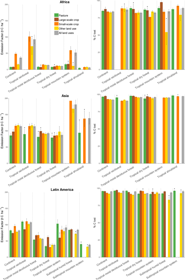
Standard image High-resolution imageAggregated EFs at the continental level (figure 5, left; table S3.1) showed that continental EFs for all follow-up land uses are lowest in the African region (8–49 Mg C ha−1). The highest continental EFs could be found in the Asian region (67–118 Mg C ha−1), while continental EFs for Latin America were positioned in the middle (74–96 Mg C ha−1). Continental EFs for small-scale croplands were higher than for pasture and large-scale cropland in all continents and higher than other land use in Africa and Asia. This same pattern can be observed across the eco-zones in Africa, and most of the eco-zones in Latin America. In the tropical dry forest of Latin America small-scale crop has the lowest EF, and in the tropical mountain system it has a lower EF compared to pasture. In Asia, eco-zone level EFs for other land use are more similar to, or in the tropical dry forest higher than, small-scale crop EFs. No clear pattern emerged for pasture, large-scale crop and other land use EFs on the eco-zone level. For all continents, EFs for all land uses tend to be higher in the tropical rainforest and the tropical mountain systems.
Figure 5. Emission factor and percentage carbon loss per follow-up land use (All land uses is combination of pasture, small-scale crop, large-scale crop and other land use), aggregated at continent and eco-zone level (All values can be found in tables S2.1 and S2.2 in the supporting information). Error bars represent standard deviations of the mean. Note: eco-zones in Latin America differ from Asia and Africa (x-axis).
Download figure:
Standard image High-resolution image
In Asia and Latin America, the percentage carbon lost (figure 5, right; table S3.2) tended to be more comparable across follow-up land uses and eco-zones than EF estimates. In Africa, the percentage of carbon lost was generally lower than in Asia and Latin America, and there was more variability.
Country-level EFs and percentage of Carbon lost can be found in tables S3.3 and S3.4.
4. Discussion
Our results show that agriculture was the dominant land use following deforestation between 1990 and 2000, but the dominance of specific agricultural land uses differed per continent. The findings for Latin America and for South East Asia are in line with previous studies that identified large-scale agriculture, increasingly producing for international markets (cattle ranching, soybean farming and oil palm plantations), as the main driver of deforestation since the 1990s (Geist and Lambin 2002, Rudel et al 2009, Boucher et al 2011, Romijn et al 2013, Stibig et al 2014). In contrast, deforestation in most of Africa is still largely due to small-scale agriculture (DeFries et al 2010, Fisher 2010, Hosonuma et al 2012, Bodart et al 2013). Small-scale agriculture is also an important factor in deforestation in Central America, the Andean region, and parts of Asia. A recent global study considering a few broad types of deforestation drivers (e.g. commodity-driven, shifting agriculture, wildfires) found a similar dominance of commodity-driven deforestation in Latin America and Southeast Asia, and of smaller-scale (shifting) agriculture in Africa (Curtis et al 2018).
Other land uses made up a considerable (>30%) part of deforested areas in Indonesia, Lao PDR and Cambodia. In Indonesia, this other land use mainly consisted of shrublands where no specific human activity could be identified. In the lowlands of Indonesia, this could partly be a consequence of the misuse of subsidies for establishing plantations (Romijn et al 2013). In the highlands of Sumatra and Borneo and in montane mainland South East Asia, these shrublands are more likely to be part of swidden landscapes (Fox et al 2014, Mertz 2009). In Lao PDR and Cambodia the other land use appeared to be linked to subsistence activities as well. Similarly, part of the other land use following deforestation in African countries could be found around villages, where fuelwood collection, grazing and fire could have caused a reduction in tree cover or a change in land use. Visual interpretation of satellite imagery is limited in its ability to identify these small-scale anthropogenic activities. In addition, deforestation areas could be under- or over-estimated in the African tropical dry forests as it is particularly difficult to map areas of open woodlands. More specifically, at low levels of tree cover densities (<30% tree cover), the distinction between forest (>10% tree cover) and other wooded land (5%–10% tree cover) is difficult to determine, which can cause errors in identifying dry forests (Lambin 1999, FAO and JRC 2012, Keenan et al 2015, Bastin et al 2017).
In Latin America the main drivers of deforestation are clearing for pastures and for large-scale crops such as soybean. Forest clearing for mechanised agriculture, associated with large-scale croplands, typically involves a more thorough removal of biomass than clearing for pasture and small-scale agriculture (Houghton 2012). Whether forest conversion to large-scale cropland or to pasture and small-scale agriculture has a higher emission factor depends mostly on the initial biomass of the forest. In Brazil, for example, forest conversion to pasture mostly occurs at the forest frontier where forests have higher carbon densities than forests in Mato Grosso State where large-scale cropland expansion mostly occurs (figure 3). In contrast, in Paraguay the EF for large-scale cropland is more than double that of pasture (table S3.3). Here, cropland expansion occurs in the tropical moist deciduous forest while pasture expansion mostly occurs in the lower biomass tropical dry forests. In the Latin American tropical rainforest eco-zone, small scale cropland often occurs in remote places with dense forests and larger-scale cropland occurs more in accessible areas with lower density forests (figure 4). The dynamics are different in the tropical dry forest eco-zone where forest clearing for small-scale cropland mostly occurs in the lower biomass dry forests of Mexico, and forest clearing for large-scale cropland in Brazil, Bolivia and Argentina. In Asia and Africa there is less difference between the EFs of the different forest conversions.
Our results show that carbon stocks of forests averaged over all sample units within an eco-zone are generally higher than the carbon stock of those forests that were cleared, for example for forest converted to pasture at the continental scale (table 3). This indicates that mean carbon stocks across an eco-zone do not always accurately represent the carbon stock of forest areas that have undergone change within that eco-zone. The use of eco-zone mean carbon stocks would introduce substantial bias (overestimation) in estimates of carbon emission from deforestation. However, considering that forest degradation is often a precursor of deforestation and that their related emissions are difficult to assess, using mean carbon stocks of all forests allows emissions from forest degradation to be captured in national estimates of carbon emissions.
Within each sample unit, we used carbon stocks of stable forests (i.e. forests remaining forests from 1990 to 2005) as a proxy for carbon stocks of forests that were cleared between 1990 and 2000 within such sample unit. Although within a sample unit, cleared forests might have had a different biomass content than stable forests (e.g. a lower value in case of previous degradation), we lack time-series of spatially explicit AGB values so we consider it to be the best proxy currently available. This highlights the need for time-series of spatially explicit data for both forest area change and forest carbon stock analyses.
In general, large uncertainties are associated with pan-tropical AGB maps, in particular in areas with few field data. However, these maps can provide reasonable carbon stock estimates when aggregated over large regions (Mitchard et al 2013). Our estimates of mean forest carbon stock of all forests within an eco-zone are lower than IPCC Tier 1 values (table S4.1), likely because they are mainly derived from average values for mature forest stands (Gibbs et al 2007). Our estimates are comparable to the alternative Tier 1 values by Langner et al (2014), except for some African eco-zones where our values were lower (table S4.1). A recent study focusing on AGBin African savannahs and woodlands show similar low AGB stocks (Bouvet et al 2018).
The IPCC Tier 1 default values assumed that all biomass is cleared when preparing land for pasture and cropland use. The default IPCC Tier 1 value for carbon stock in AGB for non-woody annual crops after one year is 5 Mg C ha−1, with a zero net accumulation of biomass carbon stocks occurring in the cropping system (table 5.9 in IPCC 2006). For grasslands, the Tier 1 total (above- and below-ground) non-woody biomass carbon stock ranges from 4.35 (dry tropics) to 8.05 (moist and wet tropics) Mg C ha−1 (table 6.4 in IPCC 2006, converted from dry matter to C). The AGB map used in this study (Zarin et al 2016) is primarily made for estimating and mapping AGB of live woody vegetation in forests. While the IPCC provides Tier 1 estimates for the non-woody vegetation, we provide estimates of the carbon stock of live woody vegetation still present after deforestation. This indicates that not all woody vegetation is cleared, or that regrowth occurs. For example up to 24% of the forest carbon stock can remain after forest conversion to small-scale cropland in the tropical dry forest in Africa (table S3.2). This study provides an opportunity to refine the default IPPC values for annual crops (table S5.1) and grassland (table S5.2).
Our EF estimates are based on historical data on deforestation (1990–2000) and biomass (2000). A study by De Sy et al (2015) illustrated that hotspots of forest conversion by specific drivers change over time and accordingly the key areas of deforestation change to lower or higher biomass forests, which would influence the emission factors. While our emission factors might be only representative for the time period studied, our results also show that emission factors are mainly determined by the initial forest carbon stock. The percentages of carbon lost seem to be more robust, and less dependent on initial forest biomass. This offers opportunities for REDD+ countries to generate local emission factors from our country or eco-zone estimates of percentage of carbon lost (tables S3.2 and S3.4). Countries should give preference to up-to-date, region- and context-specific data, but in absence of these data our estimates can provide an alternative. REDD+ countries can use good quality national forest biomass maps or inventory data to estimate initial forest carbon stocks. Our percentage of carbon lost estimates can then be applied to calculate emission factors for specific follow-up land uses. If follow-up land use is not known, we also provide estimates for all land use combined (tables S3.2 and S3.4, All land uses).
Our study highlights that information on fate of the land after forest conversion can be valuable for REDD+ policy design and implementation. It provides more insight into the spatial dynamics of land-use change and can help in attributing forest loss and carbon emissions to human activities. In addition, the co-location of data on forest loss, biomass and fate of the land provides further opportunities to link follow-up land use to other aspects such as fate of the carbon and land use management practices. We recommend that broader land use monitoring is integrated into national REDD+ forest monitoring.
Acknowledgments
This research was generously supported by the contributions of the governments of Australia (Grant Agreement # 46167), the United States Agency for International Development (Grant AgreementEEM-G-00-04-00010-00) and Norway (Grant Agreement #QZA-10/0468) to the Center for International Forestry Research. This work was carried out as part of the Consultative Group on International Agricultural Research programs on Trees, Forests and Agroforestry (FTA) and Climate Change Agriculture and Food Security (CCAFS). The authors would also like to thank Anika Paschalidou, Gijs van Lith, Sanjiwana Arjasakusuma and Prisca Masango for their contribution in the visual interpretation of the land use.
Data availability statement
The data that support the findings of this study are available from the corresponding author upon reasonable request.