

Abstract
Snow thickness measurements over relatively smooth Arctic first-year sea ice, obtained near Cambridge Bay in the Canadian Arctic (2014, 2016 and 2017) and near Elson Lagoon in the Alaskan Arctic (2003 and 2006), are analyzed to quantify physical length-scales and their relevant scaling behaviors. We use the multi-fractal temporally weighted detrended fluctuation analysis method to detect two major physical length-scales from the two independent study locations. Our results suggest that physical processes underlying the formation of snow dunes are consistent and that the wind is the main process shaping the snow thickness variability and redistribution. One scale, around 10 m, appears to be related to the formation of the snow 'dunes', while the other scale, between 30 and 100 m, is likely associated with the various interactions of the snow dunes such as merging, calving and lateral linking. Results imply that snow on level sea ice shows self-organized characteristics.
Export citation and abstract BibTeX RIS

Original content from this work may be used under the terms of the Creative Commons Attribution 3.0 licence. Any further distribution of this work must maintain attribution to the author(s) and the title of the work, journal citation and DOI.
1. Introduction
Arctic snow cover accumulation and redistribution on seasonal, first-year sea ice (FYI), which falls during from freeze up through to early summer, but does not survive more than a year, exhibits high spatiotemporal variability (Iacozza and Barber 1999), and plays a critical role in directly controlling the Arctic sea ice mass balance budget estimations (Curry et al 1995, Déry and Tremblay 2004, Leonard and Maksym 2011, Overland et al 2015). Wind-blown snow redistribution over FYI (Savelyev et al 2006) results in a heterogeneous distribution of snow thickness, with snow tending to preferentially accumulate in snowdrifts and leeward positions of morphological features such as pressure ridges, the structure of sea ice caused by the collision of ice floes (Sturm et al 1998, Iacozza and Barber 2010). Previous studies also suggest the formation of snow dunes such as barchan dunes (a crescent-shaped dune generated by prevailing winds), and transverse dunes (a long dune with a wavy ridge), are both controlled by wind speed and snow surface conditions. Their formation has been found to be similar to the formation and behavior of sand dunes, though differences exist in merging, calving and collision processes (Filhol and Sturm 2015), as well as bonding processes (sintering) (Blackford 2007). Resulting heterogeneous snow distribution patterns have been found to affect local-scale processes such as melt pond distributions during summer (Petrich et al 2012), perturbations in surface sensible and latent heat fluxes (Dery and Taylor 1996), estimates of snow precipitation from microwave remote sensing data (Picard et al 2014) and transmittance of photosynthetically active radiation affecting primary algae productivity (Mundy et al 2007).
Previous studies employed a semi-variogram based approach to estimate the spatial variability of snow cover on relatively smooth FYI, at short length scales (10–20 m) (Sturm et al 2002, Iacozza and Barber 1999, 2010). However, their semi-variogram approach could not detect other length-scales, possibly due to non-negligible non-stationarity effects contained in longer length scales. In this study, we investigate snow thickness measurements on FYI over different spatial scales to identify the main physical length scales and assess the relevant physical mechanisms determining those scales. To achieve this, we focus our efforts on the detection of exponents  from various transect measurements of snow thickness over level FYI;
  is a characteristic of the asymptotic behavior of the long-ranged spatial correlation
  However, due to multi-fractal characteristics a single exponent cannot represent the whole aspect of the physics contained in the given data, rather multiple exponents are required to characterize the data. Importantly, we will trace the change of the exponent from the snow thickness measurements in various length-scales. The value of the exponent
  and its relevant length-scale provide us with plausible conjectures of the governing physics that control snow thickness fluctuations in the length-scale.
We utilize a proven methodology called multi-fractal temporally weighted detrended fluctuation analysis (MF-TWDFA) (Koscielny-Bunde et al 2006, Zhou and Leung 2010, Agarwal et al 2012) to characterize the wind-blown redistribution of snow on smooth FYI and establish the physical length scales induced by wind. The methodology is particularly suited to our application as it minimizes the impact of non-stationarity in snow thickness data when characterizing the scaling behavior of correlations. The MF-TWDFA is a modified, extended version of multi-fractal detrended fluctuation analysis (MF-DFA) (Kantelhardt et al 2002, 2006). The MF-TWDFA uses a weighted regression approach and hypothesizes that, in any discrete time series, points closer in time are more likely to be related than distant points (Zhou and Leung 2010). The MF-DFA is designed to erase the non-stationary trends as much as possible and reveal the auto-correlated characteristics of stationary fluctuations. It contrasts with the semi-variogram  defined by half of the average of squared difference between points (
 and
and  ) separated at distance
  This has been widely used in geophysics for spatial statistics. However, the semi-variogram approach does not account for the non-stationary processes hindering detecting multiple exponents. The MF-TWDFA has previously been utilized to understand long-range correlations and multi-fractal properties in daily satellite retrievals of Arctic sea ice albedo and extent (Agarwal et al 2011, 2012). The physical length-scales detected in the MF-TWDFA and the statistical characteristics of fluctuations are the basic information underlying a core mechanism for a given phenomenon. Determining these length scales is crucial in the development of simple models containing major physics that can be utilized for new parameterizations in global climate models and stand-alone sea ice- or coupled regional-models. Here, we focus on identifying common length scales of accumulated snow on smooth FYI and suggest a mechanism based upon comparison with similar physical phenomena. Finally, we consider limitations and further research based on our findings.
2. Methods and data
2.1. Snow thickness and wind speed measurements
In situ snow thickness measurements were acquired from a relatively homogenous pan of smooth landfast FYI, located in Dease Strait (69.03°N, 105.26°W), ∼16 km south of Cambridge Bay in the Canadian Arctic. Wind speed and direction measurements were obtained from the Environment and Climate Change Canada Weather Station, located ∼5 km away from the snow thickness sampling sites. Snow thickness measurements were collected during the spring season (early April to late May) in 2014, 2016 and 2017 (figure 1 and table 1).

Figure 1. (a) Study area map of the Western Canadian Arctic and Alaska, with squares centered on Dease Strait and Elson Lagoon. Figures (b)–(f) depict snow thickness transect locations (yellow lines and crosses) collected on smooth, first-year sea ice sites at Elson Lagoon in 2003 and 2006, and Dease Strait in 2014, 2016 and 2017. Snow thickness transect locations are shown overlaid on satellite C-band Synthetic Aperture Radar (SAR) images. Figures (b) and (c) are overlaid on ERS-2 SAR satellite images, (d) on a RADARSAT-2 SAR image; and (e) and (f) on Sentinel-1 SAR images. All SAR images were acquired during corresponding snow sampling periods.
Download figure:
Standard image High-resolution imageTable 1. Snow thickness measurements made on first-year sea ice from Cambridge Bay, Canadian Arctic (2014, 2016 and 2017) and Elsoon Lagoon, Alaskan Arctic (2003 and 2006).
| Season | Transect ID | Number of measurements | Sampling intervals (in meters) |
|---|---|---|---|
| 2014 (19–22 April) | 2014T1 to 2014T20 | 5200 | 1 |
| 2016 (23–26 May) | 2016T1 to 2016T3 | 600 (T1), 500 (T2), 1000 (T3) | 5 (T1), 6 (T2), 4 (T3) |
| 2017 (01–08 April) | 2017T1 to 2017T5 | 850 (T1–T2), 366 (T3), 477 (T4), | 2.4 (T1–T2), 1 (T3-T5) |
| 468(T5) | |||
| 2003 (04–19 March) | 2003T1 | 3483 | 4 |
| 2006 (16 March) | 2006T1 | 2576 | 1 |
In 2014, 400 snow thickness measurements were recorded at 1 m intervals, at 20 different sites (named 2014T1 to 2014T20). Each site consisted of a 200 m transect parallel to the snow drift pattern, and a 200 m transect orthogonal to the drift pattern (figure 1(a)). Transect mean snow thickness in 2014 ranged from 12 to 18 cm. In 2016, four transects of varying lengths and sampling intervals were conducted parallel to, and orthogonal to, the snow drift pattern (named 2016T1 to 2016T3). Moreover, all 2016 transects were designed to transition from smooth, to moderately rough, and again to smooth FYI sub-types. Transect mean snow thickness in 2016 ranged from 12 to 22 cm. In 2017, two transects with 2.4 m sampling intervals (named 2017T1 and 2017T2), and three transects with 1 m sampling intervals (named 2017T3 to 2017T5), were conducted. Transects 2017T1 and 2017T2 were around 500 m in total length; 2017T3 to 2017T5 were around 800 m in total length. Transect mean snow thickness in 2017 ranged from 17 to 35 cm.
Our underlying assumption is that the variability in snow thickness induced by the wind-blown redistribution is an accumulated effect since sea ice freeze-up, which occurs around October. Therefore, we use the mean wind speed between October 2013 and April 2014, and likewise for 2016 and 2017 cases. Apart from varying wind speed and directions, no significant precipitation events were reported in between sampling days during all three years. Even though we knew the wind speed magnitude and direction on the snow thickness sampling dates, this is not directly related to the variability of snow thickness we measured during those dates.
Further in situ snow thickness measurements were sampled from the landfast, smooth FYI of Elson Lagoon near Barrow in the Alaskan Arctic (71.31°N, 156.48°W) during March 2003 and March 2006. Wind speed and direction measurements were obtained from the Barrow Atmospheric Baseline Observatory, located ∼5 km away from the snow thickness sampling sites. This site is mainly protected by barrier islands, leading to no significant ocean currents and exhibit similar geographical conditions to Cambridge Bay. Snow thickness was measured at 4 m and 1 m sampling intervals in 2003 and 2006, respectively. The measurements were recorded along traverse lines with the total lengths of 18.4 km in 2003 and 2.8 km in 2006. The mean snow thickness in Elson Lagoon was 12 cm. Detailed information regarding the area and the measurement methods for the Elson Lagoon data are described in Sturm et al (2006).
Cambridge Bay and Elson Lagoon are covered by smooth FYI and deformation features such as cracks and sea ice ridges were not observed, which can significantly influence snow drifts. Hence, the spatial variability of snow thickness can be assumed to be mainly controlled by wind-blown redistribution leading to snow dune formation (see the photos taken in Cambridge bay (figure S1 is available online at stacks.iop.org/ERL/14/104003/mmedia) in supplementary material). This is the major reason to choose the snow thickness data from these two areas. Due to the smooth ice surface, the local precipitation of snow and redistribution by wind are the major factors controlling the variability of snow thickness.
The mean and standard deviation of snow thickness from 2014 sampling in Cambridge Bay are 13.37 cm and 6.71 cm, and from 2016 are 11.93 cm and 7.20 cm, respectively. The mean snow thickness from 2017 in Cambridge Bay is 26.42 cm, much larger than the previous two years, but the standard deviation is similar at 8.93 cm. In Elson Lagoon, the mean and standard deviation from 2003 are 29.81 cm and 16.54 cm, respectively, and 13.70 cm and 8.8 cm from 2006 measurements.
2.2. Methodology
The spatial variability of snow thickness induced by wind is well described in figure 2, which shows several original snow thickness measurement data obtained in Cambridge Bay (figures 2(a) and (b)) and Elson Lagoon (figures 2(c) and (d)). The comparison between original data (black lines) and moving-averaged (10 m) one (red lines) suggests that there are multiple length-scales. The original data contain undulations in 10 m scales and the moving-averaged one slowly oscillate with around 50 m length-scale. These length-scales should be closely related to specific physical processes. Hence, it is necessary to detect governing length-scales systematically from the data and check out whether common length-scales are observed from various different measurements, which could lead us to have a plausible conjecture of common physics governing in wind-blown snow redistribution.
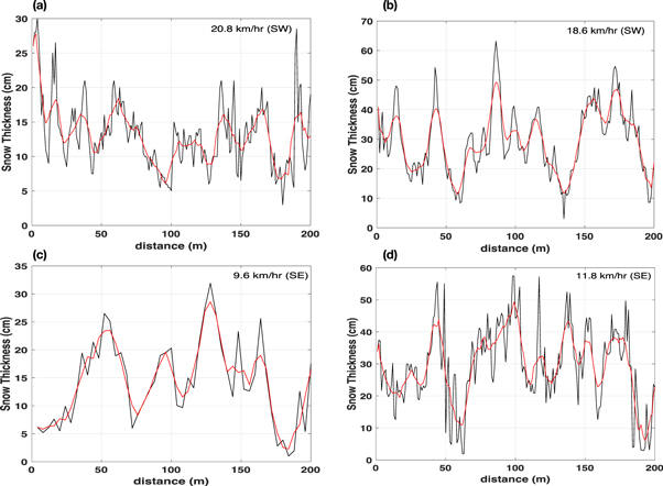
Figure 2. Examples of snow thickness measurements. Figures 2(a) and (b) shows the variability of snow thickness in a transect measurement with 1 m spatial resolution in Cambridge Bay from 2014 and 2017, respectively. Snow thickness measurements from Elson Lagoon during March 2003 and 2006 are shown in figures 2(c) and (d), respectively. The spatial resolution of the measurement at 2003 (2006) is 4 m (1 m). The red lines represent the smoothed data after applying a 10 m moving average to the original transect data. The graphs also indicate the mean wind speed and predominant wind direction.
Download figure:
Standard image High-resolution imageOne of the most common statistical quantities characterizing length-scales is the autocorrelation  where
where  is the total length of series of measurements describing the phenomenon (in time or space),
  the ith snow thickness measurement and
  is the time or length lag (here length). The associated length or time scale
  is calculated by
  where
where  implying the variance of the snow thickness measurement. When the process is short-ranged, such as
  the
the  is finite and equal to
  which is the length or time-scale for the phenomenon. However, when the process is long-ranged, i.e. the autocorrelation follows a power-law defined by
 becomes infinity, which leads to a non-Gaussian distribution for the variability and implies long-range correlated statistics. The long-ranged correlated process quite common in geophysical phenomena due to their multi-fractal structures is also expected in snow thickness data. It is indisputable that the exponent
  could be used to characterize long-ranged physical processes shaping the spatial variability of snow thickness. This idea originated from the seminal work by Hurst who investigated the variability of water levels in the Nile river (Hurst 1951).
Interestingly, one exponent  is not enough to characterize the whole aspect of one specific phenomenon. Normally, the exponent
  changes depending on the scale
  There might exist a crossover
  where the exponent
  changes from
  to
to  (Kantelhardt 2009). The change of the exponent implies the emergence of new governing physics around the scale
 This crossover is interpreted as a length or time scale associated with the major physics linking to the exponent
 There could be multiple crossovers of the exponent in a given dataset. If it is possible to robustly identify them all, it enables us to organize the scale dependency of governing physical processes. Generally, it is very challenging to obtain the multiple exponents from the direct calculation of the autocorrelation
  due to the non-stationarity in longer length-scales combined with noise.
Numerous methods have been introduced to construct the multiple correlation exponents based on power spectrum, wavelet transform and fluctuation analyses to overcome the limits of the direct calculation of the autocorrelation (Kantelhardt 2009). In this research, we rely on the MF-TWDFA, an upgraded version of the MF-DFA. The MF-DFA was designed to estimate the scale-dependent exponent  in non-stationary time-series data containing long-term trends, and has been successful in revealing the multi-fractal structure of geophysical phenomena (Kantelhardt et al 2002). The MF-TWDFA is a variant of the MF-DFA improving the robustness of extracting the scaling of fluctuations (Zhou and Leung 2010). In the MF-TWDFA, our focus lies on the scaling law represented as
  where
where  is the length-scale,
  is a constructed second order fluctuation function, and
  is the exponent identified by the slope in the plot of
  and
and  Here, the fluctuation function
  is defined as the root mean square deviation from the trend. The exponent
  is equivalent to the exponent
  with the simple relationship
  Hence,
  shows the characteristics of fluctuations in the ranges of the given length-scales, and the crossovers in the log–log plot are associated with changes in governing physics controlling the fluctuations (figure S2). Therefore, we trace the crossovers in the plot and find the slopes between adjacent crossovers. Detailed descriptions of MF-DFA and MF-TWDFA are provided in the supplementary material.
3. Results and discussions
3.1. Physical length scales
Figure 3 shows the results of the MF-TWDFA and the semi-variogram (Matheron 1963) applied to the in situ snow thickness measurements from both study locations. Results from Cambridge Bay are shown in figure 3(a), where around 30 transect measurements parallel- and orthogonal-to the main snowdrift pattern were analyzed by the second-order fluctuation function  against the length scale
  Results from Elson Lagoon are shown in figures 3(b) and (c), for 2003 and 2006 respectively.
  was constructed for each measurement and then the crossovers were located on figures 3(a)–(c) by star marks. The crossovers were classified by their locations and slopes
  which lead to two groups. The first group, marked by orange stars, is located between 0.75 (for figure 3(a)) and 0.6 (for figures 3(c)) and 1.2 in x-axis, which corresponds to a length-scale around 10 m. The second group, marked by purple stars, is located between 1.4 and 2.0, which implies a length scale between 30 and 100 m. These crossovers are boundaries between two different length-scales. However, the estimated scales near or at the crossovers dominate the variability of snow thickness following the characteristics of power laws.
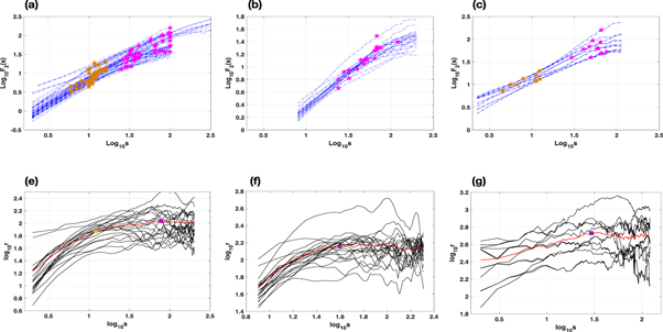
Figure 3. MF-TWDFA applied to snow transect data collected in 2014, 2016 and 2017 in Cambridge Bay (a), and to snow data collected in 2003 (b) and 2006 (c) in Elson Lagoon; plots (a)–(c) are shown as log–log plots of the fluctuation functions  (y-axis) and length scale
  (x-axis). Colored star markers represent two major groupings of positions where slopes change significantly, one near 10 m and another between 30 and 60 m. Semi-variogram applied to the same data collected in Cambridge Bay (e), and in Elson Lagoon in 2003 (f) and 2006 (g). Similarly, plots (e)–(g) are also shown in log–log plots of the semi-variogram r (y-axis) and length scale s (x-axis). The red lines represent the mean of the semi-variograms at each data set. Rectangle markers represent the major slope changes in the mean variograms.
Download figure:
Standard image High-resolution imageThe common feature in these snow thickness measurements is two physical length scales, one of which is located around 10 m and the other between 30 and 100 m. These two distinct length scales are evident in the original transect data shown in figure 2 where there are sharp peaks with 10 m length-scale and slow undulation of snow thickness with length-scales around 50 m. After applying a 10 m moving average (red lines in figure 2) to the sample transect data, the fluctuations in figure 2 around 10 m disappear, however variability around 50 m is visible.
Due to the coarse sampling intervals (4 m) of 2003 Elson Lagoon measurements, the 10 m length scale is undetectable, but the second length scales located between 30 and 100 m is well represented (figure 3(b)). In the same analysis with Elson Lagoon data collected at 1 m sampling intervals in 2006, both length scale groups are recognized (figure 3(c)). Particularly, we have to emphasize that the results from the different geographical locations are consistent under the condition that snow is deposited over relatively smooth FYI. The semi-variogram is applied to the same data and shown in figures 3(e)–(g). The results from Cambridge Bay are shown in figure 3(e) and the ones from Elson Lagoon in 2003 and 2006 are in figures 3(f) and (g), respectively. The black lines represent the results of the semi-variogram from each transect data used for the MF-TWDFA. For each black line, we find it difficult to detect the change of slope to position physical length-scales. However, the average semi-variograms (red lines) could be used to detect robust slope changes. In figure 3(e), there are two change points in the average semi-variogram, which are located at around 10 and 60 m. One change point located around 30 m is clearly detected in figures 3(f) and (g). These change points found in the average semi-variograms are consistent with the length-scales detected from the MF-TWDFA. The advantage of MF-TWDFA over semi-variograms lies on how to minimize the effects of non-stationarity contained in data. The results from the semi-variograms suffer from large fluctuations, which seem to originate from non-stationarity. However, the average of several semi-variograms provides reliable scaling laws and relevant crossovers, showing that during averaging is erased the impact of the non-stationarity. MF-TWDFA is designed to eliminate non-stationarity in calculating the fluctuation function, leading to better detection of scaling laws without significant fluctuations caused by non-stationarity. One transect measurement is enough to detect scaling laws and crossovers by the MF-TWDFA.
3.2. Governing physical processes
The next question is what kind of physical processes might be related to the two characteristic length scales: (a) 10 m, and (b) from 30 to 100 m. It is, in principle, impossible to pinpoint the exact physical processes based only on length scales. However, reasonable assumptions are provided as the basis for further investigation. First, the unique geographical characteristics of both the measurement sites are to be noted. These areas are sheltered, frozen ocean, in straits with almost no deformation of the sea ice. Deformation, if present, would influence ice surface roughness and affect snow deposition patterns. Without any notable roughness to the ice surface at the Cambridge Bay and Elson Lagoon sites, thickness variability in snow thickness should be purely due to the wind driven transport of snow particles, and not modified by surface geometry (Savelyev et al 2006).
The wind transport of snow particles generates several distinct processes such as saltation (Pomeroy and Gray 1990), suspended drift (Takeuchi 1980) and surface creep (Kind 1990). These processes have been proven to be the major processes in constructing barchan dune formations in deserts (Bagnold 1954, Kok et al 2012). Snow transport and deposition by wind is almost identical to sand except for differences in material and sintering processes only applied to snow particles (Blackford 2007, Filhol and Sturm 2015). The 10 m length-scale identified in the MF-TWDFA is highly likely associated with 'dune' formation and consistent with that in desert sand. It is known that very small sand dunes are of the order of 10 m and the most unstable wavelength growing from a flat sand surface is around 20 m (Elbelrhiti et al 2005). Furthermore, snow waves and barchan dunes obserstaved in snowfields have the length-scale ranging from 3 m to 20 m (Filhol and Sturm 2015).
The slopes from starting points to the points in the first group (orange stars) in the figures 3(a)–(c) are shown in a bar graph in figure 4(a). The slopes, which are related to the scaling of the autocorrelation, reveal the statistical characteristics of fluctuations with the given length scale in the first group (∼10 m). A significant portion of the slope values in figure 4(a) are concentrated near 1.3, which implies non-stationary characteristics with uncorrelated nature for the first group of points. For stationary long-correlated processes, the slope should lie between 0 and 1.0, but if non-stationary effects such as strong oscillations, the slope could be larger than 1.0 (Movahed et al 2006). The slopes between the first group (thick orange stars) and the second group (thick purple stars) are shown in figure 4(b). Most of the slope values are located near 1.0, which represents 1/f noise, or flicker noise (Bak et al 1987). The scaling behavior which differs by length-scales in snow was previously observed on Antarctic sea ice, Trujillo et al 2016) and terrestrial snow cover (Trujillo et al 2007). In particular, two separate length-scales on terrestrial snow were estimated using power spectral analysis (Trujillo et al 2007). The 1/f noise has previously been reported in various physical phenomena including sand piles (Bak and Chen 1991), earthquakes (Bak and Tang 1989), and ocean temperature (Fraedrich and Blender 2003), and is known to be related to critical phenomena which do not have specific scales and follow power law distributions. In the second length scale, the governing physics may be related to the interaction of the dunes, possibly by the slow movement and the merging and dispersing of the snow dunes (Filhol and Sturm 2015). In this case, where we consider the interaction of the dunes and generating 1/f noise, the best possible and simplest model to regenerate the statistical characterization shown in the field data could be a cellular automata (CA) model with threshold behavior, a critical condition for self-organized criticality (Bak et al 1987). The CA model has already been implemented for sand dunes, to simulate large-length scale sand dune dynamics (Werner 1995, Narteau et al 2009) and for terrestrial snow thickness variability (Leguizamón 2005, Collados-Lara et al 2019). Therefore, it is highly recommended to implement a CA model in snow thickness variability in this length scale. However, it is necessary to collect more evidence of the self-organized criticality in snow dune dynamics from careful further observations.

Figure 4. The slopes in the plot of  and
and  from figure 3 are represented as histograms. First, the slopes from the initial point to the point in the first group (around 10 m scale) are collected and shown in (a). Slopes between the first group and the second one are shown in (b).
Download figure:
Standard image High-resolution image3.3. Independent sampling and large-length scale variability
In previous sections, we suggested that two distinct physical processes that act to produce snow features at the two length scale ranges. It is also speculated that beyond the length-scale 60 m, the slopes shift from 1.0 to 0.5 implying white noise characteristics. This behavior is also observed in the semi-variogram analysis shown in figures 3(e)–(g). Beyond the 60 m scale, the slopes in the semi-variogram are almost flattened. If a length-scale is larger than the second length-scale, spatial autocorrelation becomes almost negligible. Therefore, it is very useful to consider the large-scale variability of snow thickness in this area from the given data.
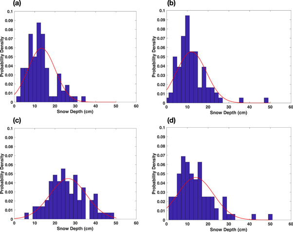
The white noise characteristics shown in the length-scales beyond 60 m suggests that samples collected at intervals greater than 60 m are statistically independent and should be close to a Gaussian distribution following the central limit theorem. The effect of the dune formation and their interactions in one area does not reach beyond this length-scale. Based on this information, we selected samples with 100 m spatial resolution. We construct two subsamples from the 2014 and 2016 data with the 100 m resolution, which are represented by the PDFs in figures 5(a) and (b). For 2017, we conducted a 100 m interval subsample from a 3.5 km transect, which leads to the PDF in figure 5(c). Similarly, we subsampled the data every 100 m from the Elson Lagoon data during 2003 for the construction of the PDF in figure 5(d).
Figure 5. Constructed probability density functions of snow thickness using subsamples collected every 100 m from transect data. For 2014 (a), two data points separated by 100 m were sampled from each transect. For 2016 (b), we subsampled the data every 100 m. For 2017 (c), we conducted a new transect with a 100 m interval. For 2003 in Elson Lagoon (d), we also subsampled the data every 100 m. Following Central Limit Theorem, the Gaussian distributions with same mean and standard deviation are shown by red curves in each figure.
Download figure:
Standard image High-resolution image
The constructed PDFs in figure 5 are approximated by a Gaussian distribution, denoting independent samples following the central limit theorem. Even though the average snow thickness is different year by year depending on the yearly weather variations, the standard deviation, which is mostly caused by wind and its interaction with snow, remains relatively consistent (section 2.1). Normally, the ratio of height to length of snow dunes is known to be around 1:70 (Filhol and Sturm 2015), which is equivalent to around 13 cm variability of snow depth for 10 m length snow dunes. This reinforces the conjecture that snow thickness variability may be controlled by the same physics, for a given ice surface type/topography (which in our case is nearly negligible for smooth FYI), regardless of the amount of annual snow accumulation. The larger standard deviation of snow thickness in Elson Lagoon seems to be understood by regional climate difference, especially the one in surface wind speed, between Elson Lagoon and Cambridge Bay. The white noise characteristics detected beyond 60 m could be useful to quantify the variability of snow thickness estimates over large spatial scales such as 100 km; the length-scale for global climate models, where the wind-based physics generating the two length-scales are impossible to be included.
4. Conclusion
Arctic sea ice is covered by snow, an efficient insulator that modulates basal ice growth during the cold winter and delays the melt during early summer. Snow thickness over sea ice is one of the most important physical quantities required to calculate the heat flux balance in sea ice. How much energy is being transferred between a sea ice-covered area and the overlying atmosphere is highly dependent upon the distribution of snow thickness in the area. From this perspective, the current research deals with the intrinsic and fundamental question regarding the major physical length scales in Arctic FYI snow thickness variability.
The FYI observation sites, Cambridge Bay and Elson Lagoon, are ice-covered ocean of almost uniform sea ice thickness; hence, the physical factors controlling snow thickness are local precipitation amounts and wind. In particular, the local variability of snow thickness is caused by the wind transport of snow particles. To estimate physical length-scales, we applied an effective multi-fractal time-series analysis method, MF-TWDFA, to snow thickness transect measurements collected in the same area in five different years.
Two major length scales are found consistently from the given data regardless of temporal and sampling-interval differences between transects. One scale is around 10 m and the other is located between 30 and 60 m. The 10 m length scale indicates short-correlated noise characteristics and the 30–60 m length scale indicates 1/f noise which implies self-organized characteristics. The physical mechanisms governing the length scales from snow covers is very similar to Barchan sand dunes in a desert. Assuming there is little difference between sand and snow in their transport by wind except their material characteristics, the 10 m length scale may be related to the formation of snow dunes by wind. The larger length-scale demonstrating the self-organized structure may be related to the collective behavior of snow dunes. This allows the possibility of simulating it using a simple CA model. Beyond a 60 m length-scale, the fluctuation almost follows white noise, which provides the justification of independent sampling for large-scale snow thickness variability. The standard deviations of snow thickness collected in different areas and during various times are similar despite different means. The standard deviations are close to the typical height of snow dunes with 10 m length, which is also consistent with that the formation of snow dunes and their interactions by wind are the main process shaping the variability of snow thickness in this area. In other similar research in the area of terrestrial snow (for e.g. Trujillo et al 2007), two length-scales were also detected, but the snow was covered with vegetation. Physical mechanisms generating the two length-scales should consider the effects of bottom roughness together with wind-blown redistribution. In our study, the flat bottom excludes the influence of bottom complexity (such as snow/sea ice interface and sea ice roughness) and only focuses on the role of wind redistributions over snow surface.
The MF-TWDFA is useful to detect several length-scales from a transect measurement. The method is designed to minimize the impact of non-stationary effects, which leads to detect change points of slope in log–log plots. The traditional method, semi-variogram, has limitations to find change points of slope in large length-scales mainly due to the undulations caused by local non-stationarities. The MF-TWDFA could be used effectively in the analysis and understanding of snow thickness distributions on sea ice, and their large- scale variability across spatial and temporal scales. The current research does not provide a geophysical basis for this second longer length-scale. Another question that should be addressed is why the range of the second length-scale is so large. It might be related to different meteorological conditions or self-organized complexity. A more thorough examination of the longer length scale should be considered in further research. Out findings confirm the usefulness of the MF-TWDFA methodology to quantify critical length scales over regional- to hemispherical-scales. Results from the current research should be a guide for further studies that include more abundant snow thickness data, possibly including airborne measurements. Relationships between length scales and wind speeds/directions should be further investigated. At the same time, model construction that will enable regeneration of variability of snow thickness as outlined in this research could be also considered as a future topic. Even though this research focuses only for relatively short spatial scales, future research should consider obtaining much longer transect data to find other length scales associated with meteorological or larger spatial scale surface roughness differences. This research is only targeted on snow covered undeformed, landfast sea ice. Governing length scales and following scaling laws should be different for snow over pack ice, where complicated sea ice surface topography contributes to significant variability in snow thickness distributions, and requires further investigation.
Acknowledgments
The authors thank Natural Sciences and Engineering Research Council of Canada (NSERC) Discovery and Tools and Infrastructure grants to John Yackel and Randall Scharien and Brent Else; Polar Continental Shelf Project (PCSP) and the Northern Scientific Training Program (NSTP) for financial and logistic support; POLAR Knowledge Canada, Cambridge Bay (Dwayne Beattie and Angulalik Pedersen) is also acknowledged for logistical support for field data collection. This work was supported by funding from the ICE-ARC programme from the European Union 7th Framework Programme, grant number 603887, ICE-ARC contribution number 065. The authors the Alaska Satellite Facility (ASF) and the Canadian Space Agency for providing RADARSAT-2 data. RADARSAT-2 Data and Products© MacDonald, Detwiller and Associates Ltd 2017—All Rights Reserved. RADARSAT is an official mark of the Canadian Space Agency.
: Data availability statement
The data that support the findings of this study are available from the corresponding author upon reasonable request. The data are not publicly available for legal and/or ethical reasons.