

Abstract
Fossil fuel combustion releases carbon dioxide into the atmosphere along with co-pollutants such as sulfur dioxide, nitrogen oxides, and others. These emissions result in environmental externalities primarily in terms of climate and air quality. Here we quantify the cost of co-pollutant emissions per ton of CO2 emissions from US electric power generation. We measure the co-pollutant cost of carbon (CPCC) as the total value of statistical life associated with US-based premature mortalities attributable to co-pollutant emissions, per mass of CO2. We find an average CPCC of ∼$45 per metric ton (mt) of CO2 for the year 2011 (in 2017 USD). This is ∼20% higher than the central Social Cost of Carbon (SCC) measure of climate damages that was used by the Obama administration in its regulatory impact analysis for the Clean Power Plan (CPP), and >8 times higher than the SCC used by the Trump administration in its analysis for the Plan's repeal. At the state-level, the CPCC ranged from ∼$7/mt CO2 for Arizona to ∼$96/mt CO2 for New Jersey. We calculate the CPCC trends from 2002 to 2017 and find a 71% decrease at the national level, contributing to total savings of ∼$1 trillion in averted mortality from power plant emissions over this period. By decomposing the aggregate and fuel-specific co-pollutant intensities into simultaneous (CO2-driven) and autonomous components, we conclude that the CPCC trends originated mainly from targeted efforts to reduce co-pollutant emissions, e.g. through fuel switching (from coal to natural gas) and autonomous changes in co-pollutant emissions. The results suggest that the overall benefit to society from policies to curtail carbon emissions may be enhanced by focusing on pollution sources where the associated air-quality co-benefits are greatest. At the same time, continued efforts to reduce co-pollutant intensities, if technologically feasible, could help to mitigate the air-quality damages of the CPP's repeal and replacement.
Export citation and abstract BibTeX RIS

Original content from this work may be used under the terms of the Creative Commons Attribution 3.0 licence. Any further distribution of this work must maintain attribution to the author(s) and the title of the work, journal citation and DOI.
1. Introduction
Electric power generation from fossil fuel combustion is a significant driver of anthropogenic climate change and degraded air quality. In the US, electric power generation was the largest single source of CO2 emissions in 2014, responsible for 39% of total CO2 emissions from fossil fuel combustion (US EPA 2016a). Although the sector has made progress in decarbonization with transportation becoming the largest emitting sector in 2016 (by a 4% margin), 35% of total CO2 emissions in 2017 were still attributable to electric power generation (US EPA 2019a). Furthermore, the electric power generation sector produced 68% of SO2, 13% of NOx and 3% of primary PM2.5 anthropogenic US emissions in 2014 (US EPA 2018a). Exposure to fine particulate matter (PM2.5) resulting from these non-CO2 combustion by-products of electric power generation, including secondary PM2.5 derived from SO2 and NOx, was found to be associated with 52 200 [90% CI: 23 400–94 300] premature deaths nationwide in the year 2005 (Caiazzo et al 2013), SO2, NOx and PM2.5 emissions were estimated to be responsible for 68%, 14%, and 16% of these impacts respectively (Dedoussi et al in preparation). Driven by fuel switching, as well as regulatory and technological changes, co-pollutant emissions from electric power generation have decreased over the past decades (Mac Kinnon et al 2018, Schivley et al 2018, Zigler et al 2018, US EPA 2019a). As a result, Dedoussi et al (in preparation) report a 50% decline in premature mortalities attributable to electric power generation between 2005 and 2011, and Lelieveld (2017) reports 35,700 [95% CI: 17 800–53 500] early deaths associated with 2015 power generation.
For the purpose of evaluating policies aiming to reduce carbon emissions, the Social Cost of Carbon (SCC), a monetized measure of the climate damages per metric ton of CO2 emissions, has been widely applied (US Interagency Working Group on the Social Cost of Greenhouse Gases 2016)5 . A full accounting of the social cost of fossil fuel combustion would include co-pollutant damages. Shindell (2015) proposed the term 'Social Cost of Atmospheric Release' to refer to the combined costs of climate and air quality damages.
The air quality externalities resulting from co-pollutant emissions have been studied from both an aggregate social cost perspective (Nemet et al 2010, Thompson et al 2014, Driscoll et al 2015) and an accountability viewpoint at the power plant level (Buonocore et al 2014, Henneman et al 2017, Henneman et al 2019). Recent research on the co-benefits (i.e. the positive health effects of co-pollutant reduction) from 'deep decarbonization' policies in the US concluded that these policies could prevent on average 36 000 premature deaths annually from 2016 to 2030, and that the monetized value of the avoided early deaths would surpass the climate benefits of these policies, as quantified by applying the US government's SCC (Shindell et al 2016). Similar findings have been reported globally (Parry et al 2014, Scovronick et al 2019), as well as regionally, e.g. for the European Union (Berk et al 2006) and China (Li et al 2018). Thompson et al (2014) estimated that co-benefits can be up to ten times as large as the carbon policy costs in the US. Since these air quality impacts are proximate in time and space to the emission source, they may command greater attention from policymakers than more distant and widely diffused climate impacts. Including them in the full social cost evaluation enables the design of more efficient multipollutant strategies (National Academy of Sciences 2004, McCarthy et al 2010, Boyce and Pastor 2013), and possibly advances equity objectives (Ringquist 2005, Mohai 2008, Zwickl et al 2014, Cushing et al 2016, Boyce and Ash 2018, Boyce 2019, Cushing et al 2018).
We are not aware of studies that analyze the trends in co-pollutant emissions, their societal cost, and the underlying reasons for these trends for US electric power generation, using comprehensive atmospheric chemistry-transport modeling. This is of particular interest as new emission control technologies and new emission regulations together with fuel switching have changed co-pollutant intensities in recent years. This paper attempts to close this gap. Specifically, we decompose the trends of co-pollutant emissions in simultaneous (CO2-driven) and autonomous components to provide insight on the drivers of the changes and the historic relationship between carbon emissions and co-pollutant emissions. As such, we can gain insights into the potential contribution of decarbonization strategies to air quality improvements. We then estimate the co-pollutant cost of carbon (CPCC) on the national level and the state level from the early deaths attributable to co-pollutants from power plants per metric ton of CO2 emissions, monetized by the value of a statistical life (VSL) as recommended by the US Environmental Protection Agency (US EPA). The analysis compares the magnitude of the air quality effects of US electric power generation (EG) to climate damages. To do so, we use standard US EPA measures for the VSL and the SCC, putting aside additional criticisms that can be raised as to the appropriateness of methodologies used to calculate the SCC (Pindyck 2013, Boyce 2018).
We perform our analysis for 2002–2017. This period has been transformational for the US electric power generation sector. Regulatory measures, including the Acid Rain Program, the NOx Budget Trading Program, and the Clean Air Interstate Rule followed by the Cross State Air Pollution Rule, targeted the reduction of co-pollutant emissions over this period (US EPA 2019b). In parallel, fuel switches, primarily from coal to natural gas, resulted in both lower carbon emissions and lower co-pollutant intensity (Lueken et al 2016, Schivley et al 2018). The results are particularly relevant in the context of the repeal of the Obama administration Clean Power Plan (CPP) and its replacement by the Affordable Clean Energy (ACE) Rule, which was announced by the Trump administration on 19th June 2019, giving states freedom in establishing standards for greenhouse gas emissions from fossil-fueled power plants (US EPA 2019c).
The paper is organized as follows. Section 2 outlines the methods and the data used. Section 3 presents an analysis of co-pollutant emission distributions and trends in the US, and the calculated CPCC of the electric power generation sector. Section 4 discusses our findings and offers concluding remarks.
2. Methods
In this paper, we define the climate and air quality social cost (CAQSC) of combustion products as the sum of climate damages per unit of CO2 emissions (SCC) and the CPCC derived from the premature mortality attributable to co-pollutants contributing to PM2.5 exposure (SO2, NOx, primary PM2.5, and NH3), monetized by the VSL, per unit of CO26 :

In this section, we develop methods to analyze systematically the emission trends that lead to changes in CAQSC over time (section 2.1) and to compute and monetize the associated damages (section 2.2).
2.1. Emissions
Emission data for CO2 and the co-pollutants SO2 and NOx from the electric power generation sector at the utility-level7 are obtained from the US Energy Information Administration (EIA 2019a, 2019b). These two co-pollutant species are responsible for >80% of electric power generation's early death impacts (Dedoussi et al in preparation). Using this data, we develop methods to estimate simultaneous and autonomous trends in co-pollutant emissions.
We start by defining each co-pollutant  's co-pollutant intensity
  as the ratio of co-pollutant emission mass,
  to CO2 emission mass:

Using this metric, we decompose annual changes in co-pollutant emissions  into (i) a carbon effect
  which results from changes in use of fossil carbon; and (ii) a co-pollutant-intensity effect
  which captures changes in co-pollutant intensity over time. This yields equation (3)

The  can further be decomposed into (i) induced changes that are contemporaneous with carbon emissions; and (ii) an autonomous component that is orthogonal to CO2 trends. For example, if regulatory policies deliberately prioritize CO2 reductions from sources with higher-than-average co-pollutant intensities, declining carbon emissions will cause induced reductions in the average co-pollution intensities. In contrast, regulatory policies exclusively targeting co-pollutant emissions would result in autonomous reductions of co-pollutant intensities. Using γ to denote the induced component in co-pollutant intensity changes, we rewrite equation (3) to

From equation (4), we infer  the simultaneous effect of changes in carbon emissions on co-pollutant emissions, which captures the direct carbon effect and the induced effect, as shown in equation (5)

To empirically decompose observed changes in co-pollutant emissions into (i) the simultaneous change of carbon emissions and co-pollutant emissions  and (ii) the autonomous change in co-pollutant intensities, we model the autonomous change as a fixed, state-specific trend parameter and
  as a proportional function of changes in carbon emissions. To consider heterogeneity in the simultaneous trends in co-pollutant emissions and carbon emissions, we estimate this for the different state clusters shown in figure 1: (a) states that decreased electricity production versus states that increased electricity production to allow, for example, for the possibility that states that increase EG prioritize cleaner sources to do so; and (b) states that decreased carbon emissions versus states that increased carbon emissions, thereby capturing potential asymmetric responses of co-pollutant emissions to changes in carbon emissions, e.g. if states that move to decrease CO2 emissions target dirtiest plants first.
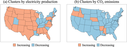
Figure 1. State clusters for the continental US, 2002–2017.
Download figure:
Standard image High-resolution imageThis yields equation (6), which is estimated for each state  and each year t

where  is the autonomous change in co-pollutant emissions in state
 is an error term with conventional properties, and
  is the state-cluster-
 -specific simultaneous CO2-co-pollutant effect. In this model,
  implies that CO2 reductions yield simultaneous reductions in co-pollutants. In contrast,
  would imply trade-offs between CO2 emissions and co-pollutant reductions. Using logarithmic first differences of emission data8
, equation (6) is estimated using weighted least squares with carbon emission weights and robust standard errors. It is estimated for both aggregate state-level emissions as well as by fuel type to capture heterogeneities in the co-pollutant trends by fuel type. The models do not set out to identify causal impacts, but they decompose trends in co-pollutant emissions into components that are contemporaneous and orthogonal with respect to carbon emissions.
would imply trade-offs between CO2 emissions and co-pollutant reductions. Using logarithmic first differences of emission data8
, equation (6) is estimated using weighted least squares with carbon emission weights and robust standard errors. It is estimated for both aggregate state-level emissions as well as by fuel type to capture heterogeneities in the co-pollutant trends by fuel type. The models do not set out to identify causal impacts, but they decompose trends in co-pollutant emissions into components that are contemporaneous and orthogonal with respect to carbon emissions.
2.2. Social cost of co-pollutants
To estimate the economic costs associated with co-pollutant emissions, we follow approaches that quantify air quality impacts through early deaths attributable to long-term effects of population exposure to fine particulate matter, PM2.5, including secondary PM2.5 resulting from SO2 and NOx emissions (e.g. Caiazzo et al 2013, Dedoussi and Barrett 2014, Fann et al 2013). PM2.5 and ozone are the most significant known causes of early deaths due to degraded air quality, with PM2.5 being responsible >85% of these for the electric power generation sector (US EPA 2011, Dedoussi et al in preparation). PM2.5 exposure has therefore become the predominant metric for quantifying the impacts of degraded air quality from electric power generation.
For estimating PM2.5-attributable early deaths, we build on Dedoussi et al (in preparation), who apply a state-of-the-art adjoint approach to trace early deaths in every state to emissions from all states in the contiguous US9 Specifically, we use source state-level early death data specific to the electric power generation sector for the years 2005 and 2011. The emission species taken into account are SO2, NOX, primary PM2.5, and NH3. Emissions data for CO2 and the aforementioned co-pollutants are obtained from US EPA's National Emissions Inventories (NEI) (US EPA 2017b, 2018b).
We quantify the CPCC for year  and state
  as shown in equation (7):

where  is the number of premature mortalities attributable to electric power generation emissions from state
  and year
  obtained from Dedoussi et al (in preparation),
  is the VSL in year
  and
and  is CO2 emissions from electric power generation reported for state i in year t. The source-wise mortality estimates include all PM2.5 premature deaths attributable to a state's emissions regardless of the state in which the deaths occur. VSL estimates are obtained following the methodology of US EPA (2014). We adjust the price level of the VSL estimates to year-2017 USD using the GDP price deflator for the US obtained from Federal Reserve Economic Data, and adjust for real income changes using per capita income growth obtained from Federal Reserve Economic Data in combination with an income elasticity of VSL of 0.7 as recommended by US EPA (2016d) and Robinson and Hammitt (2015). Consistent with US EPA practice (US EPA 2004), we use a cessation lag structure that distributes early deaths over a span of 20 years following exposure (30% in year 1, 50% in years 2 through 5, and 20% in years 6 through 20). We assume a 3% discount rate and apply CBO (2017) GDP-per-capita growth assumptions to consider future early deaths. To examine the sensitivity of our results to these assumptions, we also report results using a constant VSL. Finally, we estimate the US national timeline of CPCC between 2002 and 2017, using the NEI emission trends for NOx, SO2, primary PM2.5, and NH3 for that period and the 2005 and 2011 estimates of early deaths per unit of emission described above.
3. Results
Emissions trends are quantified and decomposed into autonomous and simultaneous components in section 3.1. Section 3.2 quantifies the CPCC and its timeline.
3.1. Emissions and trends
We start by analyzing emission distributions and trends as outlined in section 2.1. As shown in table 1, the ten states with the highest emissions by species accounted for 46%–65% of total emissions from the electric power generation sector in 2017. This concentration is partly driven by the amount of electric power generation in each state. However, differences in power generation technologies, e.g. the uptake of renewable sources, as well as different fuels, power generation efficiencies, and varying levels of emission control technologies, cause significant variation in the rankings.
Table 1. Top-10 states in share of emissions in the US electric power generation sector for 2017.
| CO2 | SO2 | NOx | Electric power generation | ||||
|---|---|---|---|---|---|---|---|
| State | US share | State | US share | State | US share | State | US share |
| TX | 12.4% | TX | 20.1% | TX | 9.5% | TX | 10.6% |
| FL | 6.0% | MO | 7.7% | OH | 5.1% | FL | 6.0% |
| IN | 4.6% | OH | 6.8% | IN | 5.0% | PA | 5.4% |
| OH | 4.5% | PA | 5.1% | FL | 4.6% | CA | 4.9% |
| PA | 4.4% | MI | 4.9% | MO | 3.9% | IL | 4.7% |
| MO | 3.9% | IN | 4.6% | PA | 3.8% | AL | 3.5% |
| WV | 3.7% | KY | 4.2% | MI | 3.6% | NC | 3.3% |
| IL | 3.7% | IL | 4.0% | NC | 3.6% | NY | 3.2% |
| KY | 3.6% | NE | 3.7% | KY | 3.6% | GA | 3.2% |
| MI | 3.2% | AR | 3.5% | WV | 3.2% | OH | 3.1% |
| CR10 | 50.1% | CR10 | 64.5% | CR10 | 45.8% | CR10 | 47.8% |
Note. CR10 = cumulative share of top-10 states.Sources. Data obtained from EIA (2019a, 2019b). Electricity generation data on net electric power generation from all fuels at the utility level.
This variation is consistent with the observed variations in co-pollutant intensities shown in figure 2. We find that, on average, 0.72 kg SO2 and 0.70 kg NOx were emitted per metric ton of CO2 released from EG for 2017, but these ratios varied among states. In general, we find co-pollutant intensities to be highest in the Midwest states, pointing towards greater use of fuels or power generation associated with higher pollution intensities.

Figure 2. Co-pollution intensities by state in kg/mt CO2 for 2017 for (a) SO2; (b) NOx. States with average annual CO2 emissions <106 t between 2002 and 2017 are not plotted.
Download figure:
Standard image High-resolution imageTurning to changes in emissions from US electric power generation between 2002 and 2017, we find a nationwide decline in CO2 emissions by 1.8%/yr. On the state-level, we observe considerable variation in CO2 trends across states as shown in figure 3(a).
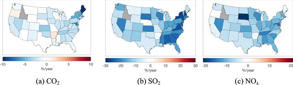
Figure 3. Trends in state-level (a) CO2, (b) SO2, and (c) NOx emissions from in-state electric power generation, 2002–2017.
Download figure:
Standard image High-resolution imageOver the same period, nationwide co-pollutant emissions declined at 13.7%/yr for SO2 and 8.8%/yr for NOx. Figures 3(b), (c) again show considerable inter-state variations in the trends. These can be attributed to a variety of reasons including decarbonization efforts, fuel switching (e.g. coal to natural gas), more stringent air pollution regulations, and advances in pollution control technologies.
To partition the observed changes in co-pollutant emissions into components that are (i) simultaneous and (ii) autonomous with respect to changes in carbon emissions, we apply the model outlined in section 2.1. The estimation results are presented in table 2.
Table 2. Summary of regression results.
| ln(SO2) | ln(NOx) | |||||||||||
|---|---|---|---|---|---|---|---|---|---|---|---|---|
| (1) | (2) | (3) | Coala | Natural Gasa | Petroleuma | (1) | (2) | (3) | Coala | Natural Gasa | Petroleuma | |
| ln(CO2) | 1.51*** (0.13) | 1.25*** (0.12) | ||||||||||
| ln(CO2) | ||||||||||||
| States with CO2 decrease | 1.57*** (0.14) | 1.25*** (0.12) | ||||||||||
| States with CO2 increase | 0.78* (0.35) | 1.12*** (0.15) | ||||||||||
| ln(CO2) | ||||||||||||
| States with electricity generation decrease | 1.45*** (0.17) | 1.55*** (0.22) | ||||||||||
| States with electricity generation increase | 1.55*** (0.18) | 1.05*** (0.11) | ||||||||||
| ln(CO2) | ||||||||||||
| Coala | 1.27*** (0.08) | 1.21*** (0.08) | ||||||||||
| Natural gasa | 0.55*** (0.14) | 0.59*** (0.09) | ||||||||||
| Petroleuma | 0.95*** (0.08) | 0.82*** (0.06) | ||||||||||

|
−0.12*** | −0.11*** | −0.12*** | −0.10*** | 0.02 | −0.11 | −0.07*** | −0.07*** | −0.06*** | −0.07*** | −0.06 | −0.08 |
| N | 731 | 731 | 731 | 672 | 720 | 730 | 731 | 731 | 731 | 672 | 720 | 730 |

|
0.46 | 0.46 | 0.46 | 0.57 | 0.21 | 0.48 | 0.51 | 0.51 | 0.52 | 0.59 | 0.31 | 0.67 |
Note. Standard errors reported in parentheses. For  the joint significance of all state fixed effects is reported as significance. Table reports weighted average of
  using CP level weights. State-level results are shown in figure 4.* Significant at 5% level** Significant at 1% level.*** Significant at 0.1% level.
aEmissions attributable to specified fuel only.
using CP level weights. State-level results are shown in figure 4.* Significant at 5% level** Significant at 1% level.*** Significant at 0.1% level.
aEmissions attributable to specified fuel only.
For the entire set of states (Model 1), a 1% change in CO2 emissions coincided with changes in the same direction in co-pollutant emission of 1.51% for SO2 and 1.25% for NOx. The elasticity >1 implies that CO2 emissions have an induced as well as direct effect on co-pollutant emissions. When we differentiate between states that reduced or increased CO2 emissions over the period (Model 2), we find states that reduced CO2 emissions to have a significantly higher elasticity in SO2 emissions than states that increased CO2 emissions. Similarly, states that reduced EG are found to have a significantly higher elasticity in NOX emissions than states that increased electricity production (Model 3). These findings are consistent with the expectation that states reducing CO2 emissions or electricity production tend to target dirtier sources first.
The autonomous co-pollutant trends by state, estimated by the parameter  are shown in figure 4. Their average values, reported in table 2, range from −12%/yr in the case of SO2 to −7%/yr in the case of NOx. In comparison, the average simultaneous CO2 and co-pollutant emission changes are smaller (−2.7%/yr in the case of SO2 and −2.2%/yr in the case of NOx).
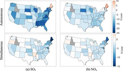
Figure 4. Average annual autonomous and simultaneous co-pollutant emission changes (%/yr) as identified by Model 1 in table 2.
Download figure:
Standard image High-resolution imageWhen we estimate the model separately by fuel type, we find that autonomous reductions in co-pollutant emissions were significant only for coal-fired power plants (−10%/yr for SO2 emission and −7% for NOx emissions). Our estimates also indicate that a 1% reduction in CO2 emissions coincided with a reduction of co-pollutant emissions by more than 1% for coal power plants only. The elasticities in the fuel-specific models are lower compared to those of the aggregated model (Model 1) since the latter captures fuel switching from coal to natural gas (figure 5) which the fuel-specific models do not.
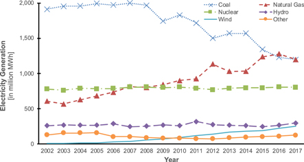
Figure 5. US electricity production at utilities by fuel type, 2002–2017. Data taken from EIA (2019b).
Download figure:
Standard image High-resolution image3.2. Co-pollutant costs (CPCs) and trends
Using the methods described in section 2, we calculate that the national-level CPCC for the electric power generation sector in 2011 was $44.7/mt CO2 (in 2017 USD). This is ∼20% higher than the IAWG SCC of $37.3/mt CO2, and ∼8 times larger than the revised SCC of $5.5/mt CO2 used by the Trump administration (both in 2017 USD), which only considers US climate damages10 . In other words, the CAQSC of combustion emissions, is found to be about 1.2 times as high as the SCC used by the Obama administration, and nearly an order of magnitude higher than the revised SCC used by the Trump administration.
Inter-state variations in the year-2011 CPCC, reported in table 3, reflect differences in co-pollutant intensity (emissions per metric ton of CO2), the dispersion of co-pollutants, background atmospheric composition, and population densities in impacted locations. Overall, the results indicate a higher CPCC in mid-Atlantic and Midwestern states. In 2011, New Jersey led the nation with a CPCC >$95/mt CO2, a result largely attributable to impacts originating from New Jersey power generation emissions on the population in New York City and environs.
Table 3. CPCC and SCC in the power sector for the year 2011 (year-2017 USD).
| Per metric ton CO2 | Per MWh of electricity generated | |||
|---|---|---|---|---|
| State | CPCC ($/mt CO2) | CPC-EG ($/MWh) | SCC-EG based on IAWG ($/MWh) | SCC-EG based on current SCC ($/MWh) |
| Alabama | 40.8 | 19.5 | 17.80 | 2.62 |
| Arizona | 7.0 | 3.4 | 17.93 | 2.64 |
| Arkansas | 27.4 | 15.6 | 21.31 | 3.14 |
| California | 48.7 | 9.7 | 7.44 | 1.09 |
| Colorado | 16.3 | 12.2 | 27.86 | 4.10 |
| Connecticut | 25.6 | 5.0 | 7.34 | 1.08 |
| Delaware | 48.6 | 29.8 | 22.89 | 3.37 |
| Florida | 21.5 | 10.8 | 18.81 | 2.77 |
| Georgia | 57.4 | 31.8 | 20.66 | 3.04 |
| Idahoa | — | — | — | — |
| Illinois | 66.4 | 30.2 | 16.97 | 2.50 |
| Indiana | 59.1 | 52.5 | 33.17 | 4.88 |
| Iowa | 44.7 | 30.3 | 25.27 | 3.72 |
| Kansas | 22.4 | 16.6 | 27.63 | 4.07 |
| Kentucky | 77.4 | 72.2 | 34.80 | 5.12 |
| Louisiana | 31.4 | 18.7 | 22.26 | 3.28 |
| Maine | 13.9 | 2.7 | 7.11 | 1.05 |
| Maryland | 49.6 | 26.2 | 19.72 | 2.90 |
| Massachusetts | 22.8 | 8.7 | 14.16 | 2.08 |
| Michigan | 67.5 | 40.2 | 22.19 | 3.27 |
| Minnesota | 43.6 | 24.3 | 20.80 | 3.06 |
| Mississippi | 35.4 | 16.1 | 17.02 | 2.50 |
| Missouri | 40.9 | 33.4 | 30.47 | 4.48 |
| Montana | 16.5 | 9.0 | 20.32 | 2.99 |
| Nebraska | 57.6 | 40.4 | 26.19 | 3.85 |
| Nevada | 8.6 | 3.9 | 17.01 | 2.50 |
| New Hampshire | 67.8 | 16.6 | 9.14 | 1.35 |
| New Jersey | 95.5 | 23.4 | 9.13 | 1.34 |
| New Mexico | 8.6 | 6.9 | 29.96 | 4.41 |
| New York | 50.4 | 12.5 | 9.23 | 1.36 |
| North Carolina | 33.6 | 17.4 | 19.39 | 2.85 |
| North Dakota | 42.4 | 35.9 | 31.58 | 4.65 |
| Ohio | 87.3 | 70.1 | 29.95 | 4.41 |
| Oklahoma | 38.0 | 25.1 | 24.62 | 3.62 |
| Oregon | 16.4 | 1.8 | 3.98 | 0.59 |
| Pennsylvania | 59.6 | 29.6 | 18.52 | 2.73 |
| Rhode Island | 61.9 | 24.8 | 14.93 | 2.20 |
| South Carolina | 42.6 | 15.6 | 13.68 | 2.01 |
| South Dakota | 67.4 | 15.8 | 8.72 | 1.28 |
| Tennessee | 57.4 | 28.8 | 18.71 | 2.75 |
| Texas | 28.6 | 17.2 | 22.35 | 3.29 |
| Utah | 13.6 | 11.1 | 30.49 | 4.49 |
| Vermonta | — | — | — | — |
| Virginia | 70.5 | 30.7 | 16.23 | 2.39 |
| Washington | 16.7 | 1.1 | 2.39 | 0.35 |
| West Virginia | 48.5 | 44.1 | 33.90 | 4.99 |
| Wisconsin | 50.7 | 34.3 | 25.20 | 3.71 |
| Wyoming | 13.4 | 11.8 | 32.67 | 4.81 |
| Nationalb | 44.7 | 23.9 | 19.91 | 2.93 |
aWe omit two states for which annual CO2 emissions were on average <106 metric tons between 2002 and 2017. bExcluding Alaska, Hawaii, and the District of Columbia.
Table 3 also reports the CPC-EG, and the SCC Emissions from EG using the SCC values from the IAWG and the current US administration (both at 3% discount rates) per megawatt-hour (MWh) of electricity produced in each state. These reflect the effects of efficiency improvements, fuel switching, and decarbonization. Some states, such as California, Maine and Oregon, had very low CPC-EG and SCC-EG, resulting from their greater reliance on non-fossil based energy sources (61% of power generation in 2017). The average CPC-EG of electricity production was relatively high in the mid-Atlantic and Midwestern states, reaching ∼$70 per MWh in Ohio and Kentucky. These states also rank high in SCC-EG by virtue of more carbon-intensive electricity production.
The ratio of CPC-EG to SCC-EG in 2011 for each state is shown in figure 6. Again we find substantial inter-state variations, with the highest ratios in the Midwest and mid-Atlantic states.
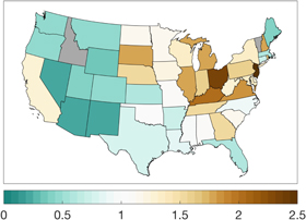
Figure 6. State-level ratio of CPC-EG to SCC-EG (based on IAWG SCC) for 2011. A value greater than 1 indicates that the CPC-EG is greater than the SCC-EG.
Download figure:
Standard image High-resolution imageWhile the CPCC was comparable in magnitude to the IAWG SCC in the year 2011, one could expect the autonomous downward trends in co-pollutant emissions to have led to significant declines in the CPCC over the period under investigation. To assess this, we compute yearly CPCC estimates averaged across all states using the method outlined in section 2.2, in combination with the year-2005 and year-2011 estimates of PM2.5 premature mortalities per unit of emission by species from Dedoussi et al (in preparation), and yearly US aggregate emission data obtained from US EPA (2016b, 2016c)11 .
The results are shown in figure 7. We find that the CPCC declined by 71% and the CPC-EG by 79% between 2002 and 2017. These outcomes can be attributed largely to the reductions in precursor emissions (section 3.1). The slightly larger reduction in CPC-EG is due to lower CO2/MWh intensities resulting from grid decarbonization, fuel switching (see figure 5), and efficiency improvements.

Figure 7. CPCC and CPC-EG, 2002–2017. The time-varying VSL is calculated using a 3% discount rate and a 0.7 income elasticity. The upper uncertainty limits in 2005 and 2011 indicate the values with a 1% discount rate and a 1.4 elasticity, and the lower uncertainty limits indicate the value with a 7% discount rate and zero elasticity. Due to the lack of state-level data for 2017 CO2 emissions, we use the 2016 state-level value scaled by the national-level change between 2016 and 2017.
Download figure:
Standard image High-resolution image
If we compare the excess mortality associated with co-pollutant emissions to that in a counterfactual scenario where the CPCC and CO2 emissions remained constant at 2002 levels, we calculate using the time-varying VSL that the savings resulting from reductions in co-pollutant emissions at power plants amounted to ∼$1.01 trillion (in 2017 USD) over the sixteen-year period.
4. Discussion and conclusions
We report the CPCC, defined as the monetized value of early deaths attributable to co-pollutants per unit of CO2 emitted, for the US electric power generation sector. For this purpose, we use EPA's VSL guidance to facilitate comparisons with the SCC used by the federal government. We find a year-2011 US average CPCC of ∼$44.7/mt (in 2017 USD), which is ∼20% larger in magnitude than the SCC used by the Obama administration (US Interagency Working Group on the Social Cost of Carbon 2016) and more than 8 times larger than the SCC used by the Trump administration in the regulatory impact analysis for its repeal of the CPP (US EPA 2017a, US EPA 2019c).
The CPCC varies at the state level, ranging, in 2011, from ∼$6/mt for Arizona to ∼$92/mt for New Jersey. While the climate benefits of reducing CO2 emissions are largely the same for all pollution sources, their air quality co-benefits can vary greatly across states and power plants due to differences in co-pollutant intensities, the transport and fate of co-pollutants, and population densities in impacted locations. From a policy standpoint, these state-level differences in the CPCC highlight the importance of considering spatially disaggregated air quality impacts in climate policies. The co-benefits of reducing CO2 emissions are substantially larger where the CPCC is greater. We note, however, that the impact of population on the CPCC poses a normative question as to whether and to what extent regulators should allow air quality to vary across locations on the basis of population density.
These results are relevant for the impact assessment of the repeal of the CPP and its replacement with ACE, which allows states to establish performance standards for fossil-fueled power plants greenhouse gas emissions (US EPA 2019c). Continuing efforts to lower co-pollutant intensities (co-pollutant emissions per mass of CO2), and with them the CPCC, would mitigate the air-quality damages of the repeal. It is possible, however, that further reductions in co-pollutant intensities beyond those achieved over the period considered in this study may be more difficult to achieve as the number of coal-fired units and the number of older units with less stringent post-combustion controls decline.
The state-level CPCC is an average across different types of power plants in each state. The air quality co-benefits of decarbonization pathways will vary depending on the replaced and new technologies, including fuel type and post-combustion processing, as discussed in section 3.1. Further research could focus on the different power-generation technologies within states and the co-pollutant effects of specific pathway changes.
Our estimates of the CPCC can be considered a lower bound in that they omit (i) costs associated with non-fatal illnesses (morbidity cost), which has been estimated broadly as a 10%–15% mark-up over mortality costs by Hunt et al (2016), and short-term health impacts; (ii) costs associated with long-term exposure to ozone, which is estimated to be 1/12–1/30 of the PM2.5-attributable early deaths (Caiazzo et al 2013, Dedoussi et al in preparation); (iii) costs associated with other combustion-related hazardous air pollutants (e.g. mercury); and (iv) other environmental impacts such as acid precipitation (US EPA 2009) and effects of air pollution on crop yields and forest growth (Ashmore 2005). Estimating the magnitudes of these additional impacts is beyond the scope of this paper and is left for further research.
Acknowledgments
The authors are grateful to three anonymous reviewers for helpful comments and suggestions. This research was supported by the Institute for New Economic Thinking (INET) Grant No. # INO15-00008, and the VoLo Foundation. This publication was in addition made possible by US EPA grant RD-83587201. Its contents are solely the responsibility of the grantee and do not necessarily represent the official views of the US EPA. Further, US EPA does not endorse the purchase of any commercial products or services mentioned in the publication.
Data availability statement
Data sharing is not applicable to this article as no new data were created or analyzed in this study.
Footnotes
- 5
As of 2014, the SCC was used by US government agencies in more than 40 regulatory impact analyses (US Government Accountability Office 2014). In 2016 the US Interagency Working Group on the Social Cost of Greenhouse Gases began using SC-CO2 as an abbreviation for the SCC; we retain the SCC notation (US Interagency Working Group on the Social Cost of Greenhouse Gases 2016).
- 6
A more complete accounting of the full cost of fossil fuels would also include the external costs of ozone exposure human health impacts, methane release, water pollution, land degradation from fossil fuel extraction, non-health impacts of air pollution, and internal costs to fossil fuel producers, as well as the climate impacts of co-pollutants. We also note that the co-pollutants have climate impacts, with SO2 and NOx having a net cooling effect, and black carbon (BC, a component of primary PM2.5) a warming effect. Using values from Shindell (2015), we estimate that the climate impacts of co-pollutants for the US electric power generation sector (SO2, NOx, BC and CH4) are <5% of CO2 impacts. They are therefore disregarded in this paper.
- 7
In this paper, emissions and power generation data from commercial and industrial power generation are not considered to restrict the analysis to the utility-level.
- 8
First differencing of all series mitigates econometric concerns as time series are found to be integrated of order one.
- 9
The uncertainty in the health impacts calculation of the premature mortality estimates is ∼±35% for the 95% confidence interval, which translates to corresponding uncertainty in the CPCC.
- 10
The IAWG year-2011 SCC value at a 3% discount rate ($32/mt CO2 in 2007 USD) is adjusted to year 2017-USD using the GDP implicit price deflator. Based on US EPA (2017), we use the Trump administration SCC at a 3% discount rate for consistency with the central value used by the IAWG.
- 11
To estimate the CPCC yearly for each state, we assume premature deaths per unit of emission to remain constant per species and state for 2002–2005 and for 2011–2017, and interpolate deaths per unit emission linearly between 2005 and 2011. These results take into account socio-economic changes, such as population changes and VSL changes, between 2005 and 2011, changes in atmospheric composition between 2005 and 2011 resulting from the impacts of emission reductions in electric power generation and other anthropogenic and biogenic emissions, and meteorological differences that altered the atmospheric sensitivity of PM2.5 formation (and thereby population exposure) with respect to a unit of precursor emissions.