


Abstract
To deal with climate change, cities must reduce their greenhouse gas (GHG) emissions and at the same time mitigate climate impacts associated with the physical infrastructure of the built environment. One strand of literature demonstrates that compact cities of sufficient density result in lower GHG emissions in the transport and the buildings sectors compared to sprawled cities. Another strand of literature, however, reveals that compactness hinders climate adaptation by amplifying the urban heat island (UHI) effect. As a result, mitigation and adaptation objectives of cities appear to contradict each other. Here, we develop a geometrical optimization framework and model of a three-dimensional city that minimizes this conflict. It makes use of the observation that low-carbon efficient transport can be realized via linear public transport axes, and that GHG emissions and UHI effects scale differently with varying geometric properties, thus enabling design that reflects both the economics and the climate of cities. We find that star-shaped cities, in contrast to radially symmetric cities, are well suited to alleviate the problematic trade-off. We also demonstrate that urban design considerations depend on transport fuel prices. The results are of particular importance for city planners of rapidly urbanizing cities in Asia and Africa who still have the potential to shape urban layout.
Export citation and abstract BibTeX RIS

Original content from this work may be used under the terms of the Creative Commons Attribution 3.0 licence. Any further distribution of this work must maintain attribution to the author(s) and the title of the work, journal citation and DOI.
Introduction
From July to August in 2013, Eastern China suffered from a serious heat wave. As temperatures failed to fall, nearly 700 people were hospitalized due to direct heat-related illness in the coastal city of Ningbo alone (Bai et al 2014). During these weeks, record temperatures were observed, especially over metropolitan areas (Wang et al 2017). A high occurrence of heat-related morbidity in cities is no surprise: already high temperatures are exacerbated in urban regions, due to the so-called urban heat island (UHI) effect (Oke 1973). Chinese cities, similar to their counterparts in other regions of the world, are hence motivated to plan urban areas that mitigate such heat wave events.
At the same time, municipal actors in Chinese cities are also working to mitigate climate change in their cities (Westman and Broto 2018). In fact, urbanizing regions in Asia, and especially China, will play an important role for climate change mitigation due to their scale and their ability to still influence urban planning (Dhakal 2009, Creutzig et al 2016).
Unfortunately, urban form that reduces greenhouse gas (GHG) emissions conflicts with urban form that reduces the UHI effect. Studies unambiguously demonstrate that more compact cities reduce not only urban transport but also building GHG emissions (Mindali et al 2004, Baur et al 2013, Baiocchi et al 2015, Creutzig et al 2015, Borck and Brueckner 2018)4 . Hence, it seems that the goal of low-carbon cities (compact cities) contrasts with the goal of cities that are resilient to heat waves (non-compact cities). In other words, there is an apparent trade-off between climate change mitigation and adaptation, specifically between heat experienced and urban transport GHG emissions.
There is, however, a possible solution. For transport and UHI, the precise compactness issues are different. For low-carbon transport, it is important to have short distance, high street connectivity, and sufficiently high population density to support massive public transit systems (Bongardt et al 2013, Ewing and Cervero 2017, Stevens 2017). For the UHI, compactness is measured as fractal dimension, and cities that have low fractal dimension and high anisotropy—stretched rather than circular cities—display a lower UHI (Zhou et al 2017), even as a multitude of other local climate factors remain equally important (see appendix). This distinction points to opportunities to balance the apparent trade-off, and led us to ask how urban form could be designed to lower both transport GHG emissions and the UHI effect simultaneously.
In response to this dilemma, we posit that star-shaped cities, organized around linear transport axes, can simultaneously address the conflicting constraints imposed by UHI and transport GHG emissions, if well-designed. We take inspiration from the city of Curitiba, Brazil, which has been developed along high-density linear transport axes, while maintaining green spaces and natural parks between and around these settlement structures (Rabinovitch and Leitman 1996). A similar design also provides the necessary density and level of amenity to move away from car-dependency in cities (Newman and Kenworthy 2006).
In the following, we first review geometric consideration of urban design, before introducing our simple urban economic model. This allows us to explain the computation of transport GHG emissions and the UHI effect. We find that UHI and urban transport GHG emissions are a function of transport costs and the number of linear transport axes. We then discuss the empirical relevance of our findings and offer two contrasting examples—Curitiba and Houston—to discuss how different types of cities can respond to the coupled climate mitigation and adaptation challenge.
Background: geometric considerations of urban design
We start with outlining geometric considerations of cities that are relevant to inform our model. For this, we consider transport GHG emissions, and UHI effects as relevant dimensions. Notably, mitigation of UHI sits at the intersection between climate change adaptation and mitigation. Reducing urban heat effects belongs to adaptation. But some strategies, such as air conditioning, heat up urban space, which in turn further augments demand for air conditioning, and consequently increase underlying energy use and GHG emissions. Hence, urban planning based strategies to reduce urban heat effects simultaneously support climate mitigation and adaptation (compare with Georgescu et al 2015).
Rationale for linear transit axes
Mass rapid transit (MRT) is the most efficient means of transport in a city. However, MRT requires high infrastructure investments and is only financially viable where sufficiently high population density supports high ridership (Cervero 1998, Creutzig 2014). From this understanding, urban economic models demonstrate that inner-city transport should be dominated by MRT, unless very low gasoline prices enable a hollowing out of city centres (Fujita 1989, Creutzig 2014). Urban economic models, however, commonly assume a radially symmetric city, the so-called monocentric model, ignoring that MRT is organized along linear axes, providing unequal access not only with radial distance but also with circular angle. A monocentric model also contrasts with the intuition of urban planners, who prefer high population density along linear MRT axes but low density away from these axes. Surprisingly, these kinds of considerations are absent in the standard literature on the economics of urban transport (Small et al 2007).
While linear transit axes can be found in cities world-wide, a few examples stand out. Copenhagen, Denmark, is well known for its finger plan of public transit and its transit-oriented development (Knowles 2012). Similarly, the example of Curitiba, Brazil, illustrates the benefits of developing the city along structured transport axes. In the 1970s, at a time of rapid urban expansion, city planners in Curitiba decided to prioritize meeting the population's mobility needs over individual motorized transport (Rabinovitch 1992). The city's development followed a master plan, which had five key principles (Friberg 2000): (i) change the radial urban growth trend to a linear one through integrated land use, road network, and transport strategy; (ii) reduce congestion in the city centre and preserve its historical buildings and neighbourhoods with legislation and economic incentives; (iii) control and manage demographical development; (iv) support urban development with economic measures; and (v) improve infrastructures.
The first principle led to the concurrent establishment of linear structural axes. Each axis has a threefold hierarchy, as illustrated in figure 1 (Rabinovitch 1992): the central road has two exclusive bus lanes for express buses, called bus rapid transit (BRT). The reason for the choice of buses—rather than trams or subways—is the significantly lower initial investment costs. Adjacent to these are two local roads. One block away, one on each side, are high capacity free-flowing one-way streets, one for traffic flowing into the city, the other for traffic flowing out of the city (Rabinovitch 1992). Land-use regulations encourage high density along these axes. By the turn of the millennium, Curitiba had been following this plan for 30 years. The benefits had become manifest: While being the city with the highest number of cars per capita amongst major Brazilian cities (Rabinovitch 1992), Curitiba also has the highest share of commuters using public transport (75% on weekdays) and its fuel consumption is 30% lower than in eight comparable Brazilian cities (Friberg 2000). Curitiba also preserved green spaces with an environmental program that greatly increased the number of parks and forested areas within the city (Gandara and Mills 2016)5 .
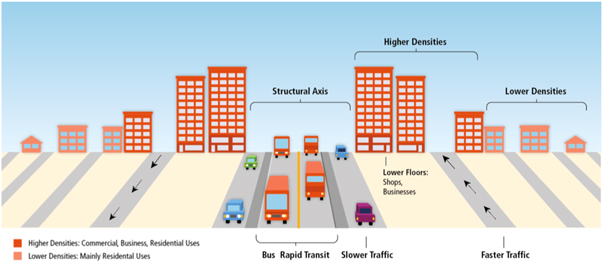
Figure 1. Curitiba's stylized trinary road system. Mixed land-use regulations allow developers to increase building heights, and add density to the corridor. The figure is based on IPCC figure 12.19 from Seto et al 2014.
Download figure:
Standard image High-resolution imageUHI geometry
Urban form characteristics partially explain the UHI effect (Zhou et al 2017, Xu et al 2019). An UHI is an urbanized area that is significantly warmer than its surrounding rural areas (see appendix). This phenomenon emerges from the thermal bulk properties and radiative forcing of urban sealed surfaces, such as asphalt, but also from the waste heat generated in cities, e.g. from automobile exhaust and air conditioning, but also from local climate conditions.
Urban from decisively shapes the UHI. From a macro perspective, the UHI scales with the logarithm of population size (Oke 1973). More specifically, powerful land-use data and computed metrics further reveal geometric features relevant to the UHI, such as city size, compactness, and anisometry (Zhou et al 2017).
Unsurprisingly, the bigger a city, the more intense the UHI. Also, more compact cities have higher UHI. As a measure for the compactness of a city, the study authors use the city's fractal dimension, a measure of how much the urban boundary line approaches being a two-dimensional object (approaching fractal dimension 2) or a one-dimensional object (approaching fractal dimension 1).6 The higher the fractal dimension, the more compact the city. The empirical analysis also showed that higher fractal dimension correlates with higher UHI intensity, suggesting a more compact city heats up more (see appendix for a qualifying view).
Another measure is anisometry: if an ellipsis is circumscribed around the city, the anisometry is the ratio of its major to its minor axis. The cited study (Zhou et al 2017) finds that the smaller this ratio, the stronger the UHI. This means that the more circular the ellipsis is, the stronger the UHI is too. In summary, the UHI is fuelled by larger cities with more population that are compact and round, while linear cities stay cooler, in the absence of other environmental or social forcing factors (as discussed in the appendix).
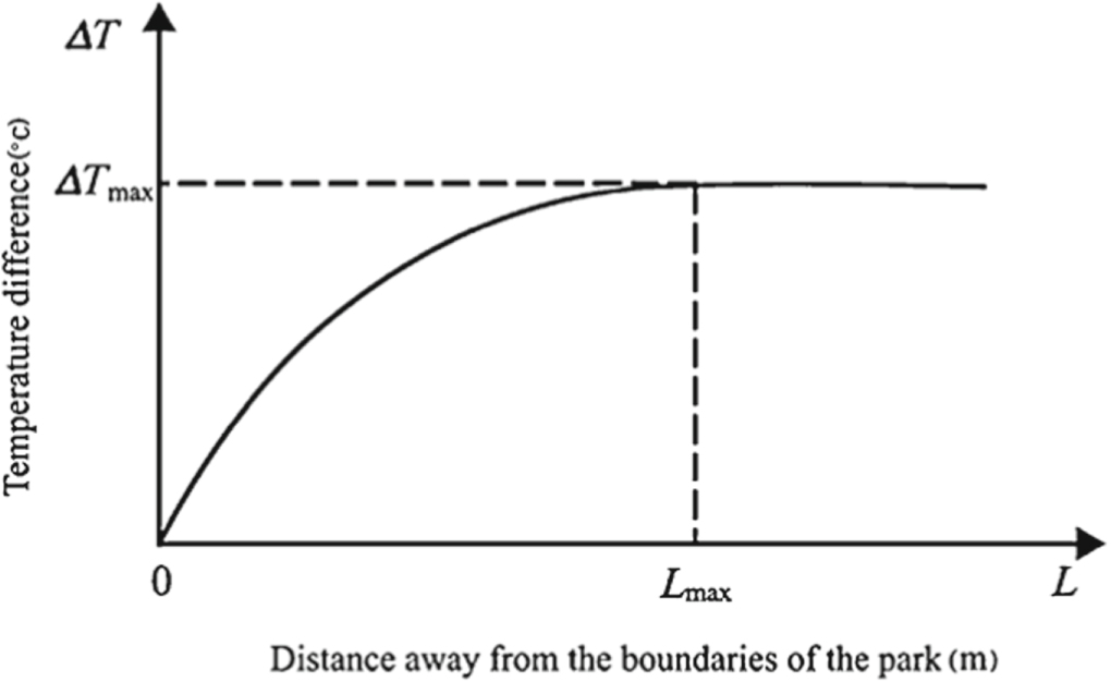
This macro perspective correlates with a micro-perspective that emphasizes different metrics and investigates what kind of park variables have what kind of impact on cooling the surrounding urban landscape. A key result of these studies is that cooling effects reach into urban surroundings as long as the park's width (Spronken-Smith and Oke 1998). Specifically, the difference between average temperature in the park TPark and temperature away from the park at distance L increases up to the maximal cooling distance Lmax (Cheng et al 2015, Lin et al 2015), as depicted in figure 2. This observation allows us to model the specific spatial dimension and geometric properties of a city on the UHI effect.
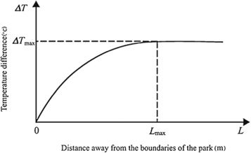
Figure 2. Temperature difference ΔT between park temperature and built-up area temperature increases as a monotone function of distance, up to the maximal cooling distance Lmax, after which the park does not cool the city any more. Reprinted from Lin et al 2015, Copyright 2015, with permission from Elsevier.
Download figure:
Standard image High-resolution imageModel mechanics: optimizing a star-shaped city
The investigated geometric considerations suggest that a city structured along linear transport axes might address both climate mitigation and adaptation concerns. We now proceed to model a star-shaped city, organized along radially outward pointing transport axes, and to compute the trade-off between UHI and urban transport GHG emissions. The key idea of the star-shaped city is its potential for reduced compactness (high accessibility to green areas reducing the UHI) combined with high density (along transit corridors, enabling low-carbon transport).
As instrumental variables, we compute the resulting UHI effect integrated over all built-up area based on the park cooling model and total transport-related GHG emissions. We then optimize the number of axes as function of the relative importance of climate mitigation (GHG emissions from transport) and climate adaptation (lowering the UHI). Finally, we consider the role of marginal transport cost, a crucial urban economic variable shaping urban form.
Transit geometry
The example of MRT that we are working with in this study is BRT (Cervero and Dai 2014), corresponding to the Curitiba example. BRT is a high capacity MRT system, but at much lower financial requirements compared to, for example, a subway system.
Length and width are the key geometric properties of the linear transit axis. We model a city that encourages settlements near the transit axis, while aiming to preserve green spaces in between. With public transport serving the axis, a restriction on the width of settlement on either side of a transport axis comes from the acceptable walking time to a public transport stop. If 10 min is an acceptable time for this walk and if average walking speed is 4.5 km h−1, then the maximum acceptable distance to walk is 800 m (Bertaud 2004). The actual spacing of bus stops for different cities around the world ranges from 200 to 600 m (Ibrahim and Isma'il 2013). As there is a trade-off between ease of access and speed of transport, the optimal bus stop spacing depends on the structure of the city and the kind of transport. For a BRT system, average station spacing in North America ranges from 0.32 km (Cleveland) to 5.28 km (Halifax) (APTA Bus Rapid Transit Working Group 2010). These distances include express portions of the system (with a maximal spacing of 12.4 km between two stops for Halifax). In Curitiba, the average residential location is less than 200 m from the next regular bus stop, but on average 1850 m away from the next BRT station (Hino et al 2014). However, these stations are highly attractive: the presence of at least two BRT stations within 500 m radius induces significantly higher walking than in the case without BRT station (Hino et al 2014).
To calculate an adequate width of linear transit axes, we consider a transit stop spacing of 1000 m along the transit axis. Then the furthest point from any station is given by

where x is the uniform width of the axis. Now, supposing that there is a diagonally walkable path from this point, y ≤ 800 m allows residents to reach a transit station in 10 min (see above). Solving for x, we find that:  ≈ 625 m. Consequently, if stations are spaced at 1 km along the transit axis and there are diagonal streets linking these stations to the furthest points (which correspond to the corners of the square with side length 1000 m centred at the stations), then the distance of transit axis to green space is 625 m. This is illustrated in figure 3, where the total width of the axis is 1.25 km, independent of the number of axes. In contrast, the length of the axis, as illustrated in figure 3, depends on the number of axes k, as discussed in the paragraph below, and the transport costs m.

Figure 3. Illustration of the star-shaped city. Cities with four, five, and six transport axes are presented for illustration. The length l(k, m) depends on the number of axes, as discussed in the paragraph 'A non-radially symmetric Alonso–Muth–Mills Model'. The width of an axis is fixed to 1.25 km, in accordance with our calculations of station spacing.
Download figure:
Standard image High-resolution imageA non-radially symmetric Alonso–Muth–Mills (AMM) Model
Our study is based on the classical monocentric urban model of AMM (Fujita 1989), which we modify by imposing linear transport axes, as inspired by Curitiba (figure 3), instead of radial symmetry. The AMM model assumes a unique city centre, to which all residents commute. It is described in detail by Fujita (1989) and summarized by Lohrey and Creutzig (2016) as follows: all residents have the same, fixed income Y, which they spend on transport costs m(r), rent R(r)s(r), and bread-consumption z. This gives the constraint:

where r is the distance from the city centre, R(r) the per-area rent, and s(r) the dwelling space. Note that m(r) is linear in radial distance, i.e. m(r) = nr for some constant n. The utility function is maximized by the residents and supposed to take a log-linear form (Fujita 1989):
This is a Cobb–Douglas function that satisfies a set of assumptions about the utility function: it is continuous, increasing for all z > 0 and s > 0, and all indifference curves are strictly convex and smooth (Fujita 1989). In the case of a closed city, i.e. constant urban population N, bid rent Ψ(r) and population density ρ(r) are described as:

In this model, the utility u is constant over r and can therefore be dropped. The transport costs m(r) are purely pecuniary costs. The bid rent Ψ is defined as the maximum rent per unit of land the household can pay for residing at distance r while having utility u (Fujita 1989). It is assumed to be equal to per-area rent R (Fujita 1989, Lohrey and Creutzig 2016). We use m(r) for transport costs if we want to stress dependence on the distance from the city centre, but most of the time we will simply use m.7
To calculate the population density ρ in this modified model, we assumed that, for a given number k of axes, each axis would host an equal fraction Nk of the overall population N. That is:  . This means that no residents live in the city centre, corresponding to the idea of the city centre as a central business district typically assumed in AMM models. The AMM model with radial symmetry allows us to determine urban radial extension. With linear transport axes, radial symmetry is lost and the residents have to be distributed accordingly onto the linear axes, subject to the density function. As result, both the number and length of axes are endogenous to transport costs and weighting of UHI. This is calculated through an iterative process. With a fixed width, fewer transport axes mean less space onto which the residents can be distributed and the axes therefore have to be longer. Accounting for this difference to the radially symmetric AMM model, we followed the same iterative method as in Lohrey and Creutzig (2016). The model is based on code originally written by Steffen Lohrey and can be found here.
Modelling UHI
We make use of the empirical insights discussed in the previous section to design a model of micro-scale UHI as a function of location and distance to green area. With the description from (Lin et al 2015) (visualized in figure 2), we fit a curve to the data from Cheng et al (2015), which provides the maximal temperature difference together with the maximal cooling distance. We find a function F that describes how the temperature increases away from the park. The cooling extent depends on the size of the park and corresponds roughly to the width of the park. While wind direction has a non-negligible influence on the cooling extent, we omit this aspect in favour of simplification (but see the appendix for details). We specifically assume that Lmax = w(r) where w(r) denotes the width of the park at any point on the transport axis at distance r from the city centre, as illustrated in figure 4. Due to symmetry, any point on the transport axis at distance r from the city centre can be express as Q = (x, r). Then, the x-coordinate indicates how far Q is from the closest park. Consequently, we obtain the following function H for the UHI effect:
where ΔTmax denotes the maximum temperature difference between city and rural area and ω denotes the width of the transport axis. At the same time, a general, exponential temperature decay away from the city centre can be observed (Zhou et al 2015). In our case, this decay happens along r-direction, the temperature decays exponentially. The function F(x) then takes the form:
F is thus the combination of the two cooling effects: in the x-direction it is the park cooling effect, where the values for ν and μ are obtained through the curve fitting explained above. In the r-direction it is the exponential decay away from the city centre.
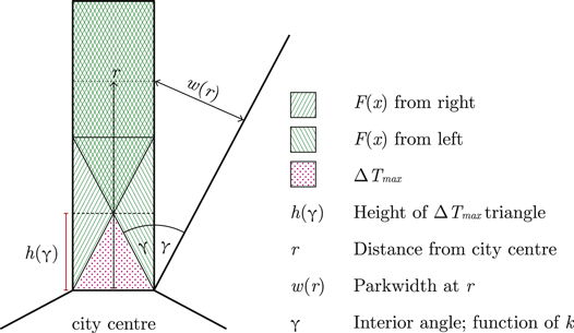
Figure 4. The park cooling effect at a point on the transport axis depends on the width of the park w(r) at that point, which in turn depends only on the distance from the city centre, r. Parks on both sides are cooling the transport axis. There is a triangle that is not cooled from either side. Its height depends on the interior angle γ, which in turn depends on the number of transport axes k.
Download figure:
Standard image High-resolution imageBasic trigonometry allows us to express w(r) as a function of the interior angle γ, which in turn depends on the number of axes k. In this way, we obtain a relationship between the UHI effect and the number of transport axes. With an increase in the number of transport axes, the park size and in particular the park width decreases. Therefore, as illustrated in figure 4, the cooling extent decreases thereby augmenting the UHI effect.
At the city centre edge of the transport axes, there is a part that is not entirely cooled by the park (figure 4). While the vertical sides of the transit axes are cooled by the park (here F(x) applies), h(γ) denotes the part of the axis that is not entirely covered by the cooling effect. Note that since γ depends on the number of axes k, so does h. In particular, the higher the number of axes, the smaller γ and hence the larger h(γ). The triangle dotted in red in figure 4 is not cooled at all, denoted with ΔTmax.
Calculating emissions from transport
The total transport emissions in the city are calculated after Lohrey and Creutzig (2016) as

In this model the relevant factors are: (i) length of axes l; with constant population N, the length of axes depends on the number of axes; (ii) number of axes k; and (iii) density profile ρ(r). We assume a direct commute along the transport axes to the city centre, ignoring the time costs of walking (which are endogenously compensated by lower residential costs).
We can then calculate the total UHI effect (abstracting from wind direction, local vegetation cover, and other specific effects) along an axis by integrating the function of equation (6) over the entire axis. Thus we have:

Here, rc is the outer limit of the city, and ω denotes the width of the axes. The integral starts at 1, as we are only calculating the UHI effect along an axis here, not in the city centre.
To compute the overall total UHI for the entire city, we simply add the number of axes times the axis-specific UHI effect in equation (8) plus the UHI effect in the city centre. The UHI in the city centre is assumed to be constant via the above formula for H(Q) and depends only on the area of the city centre. Note that an increase in the number of arms k means an increase in the area of the city centre, since this is assumed to be a regular k sided polygon with side length 1.25 km. This sum gives us Hint, the UHI effect in the city.
Having calculated the accumulated UHI effect, we need to normalize with respect to area to measure the average UHI effect felt:

Here, A is the Area of City, which denotes that part of the city that is actually built-up, including the axes and the city centre, but not the parks in between the axes. Since the density profile ρ depends on the costs of transport, we ran the calculations for various values of transport costs. The results can be seen in figure 5. As is expected, more transport axes result in an increased integrated UHI effect. At the same time, CO2 emissions are reduced by more transport axes. Increased transport costs mean more people will locate closer to the city centre, and population density increases. The calculations reflect that if the transport costs are higher, overall CO2 emissions are lower and integrated UHI is higher for the same number of transport axes.
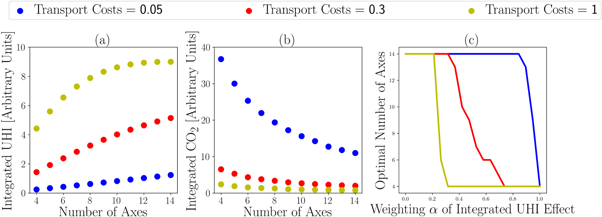
Figure 5. The balancing of UHI and GHG emissions from urban transport depends on transport costs and on the number of transit axes. We have configured the AMM model with fixed income Y = 12, fixed population N = 2, and ζ = 0.7, η = 1 − ζ = 0.3 in the calibration of the utility function. Each panel then compares different transport costs: 0.05, 0.3, and 1. The first calculates the integrated UHI as a function of the number of axes, the second the integrated CO2, and the third calculates the optimal number of axes according to the weighting given to the UHI effect as discussed in the final paragraph of the section 'Calculating Emissions from Transport'. The units here are relative units.
Download figure:
Standard image High-resolution imageIn order to determine the optimal number of transport axes, we use the optimization function:

Because both Hint and  depend on the number of axes k as well as on the transport costs m, this function does as well. The factors α, β weight the relative importance of UHI reduction (climate adaptation) and transport energy reduction (climate mitigation), respectively, with α + β = 1.
Results: optimal number of transit axes
Here we show that the number of transit axis (provided that population is constant) impacts UHI and GHG emissions from transport. Optimal city design, inversely, involves the number and length of transit axes as a crucial consideration.
Firstly, both UHI and transport emissions change with the number of axes. Specifically, with more transit axes, the UHI increases (figure 5(a)), while total GHG emissions decrease (figure 5(b)).
Secondly, we calculate how the optimal number of axes changes as a function of the weighting factor α for several values of m (figure 5(c)). This is done using the optimization function in equation (10) with several values of m (m = 0.05, 0.3, and 1, respectively). We take twenty equally spaced values for α between 0 and 1 and calculate the sum in equation (10). For a fixed m and a fixed α, we compare the results for each number of axes k. The k with the lowest G(k, m) then gives us the optimal number of k for a given m and a given α. A higher value of α means that the UHI effect becomes more important. Consequently, the ideal number of axes is lower. Conversely, with low α, the UHI effect is negligible and the optimal number of axes increases to minimize CO2 emissions from transport.
Transport costs play a crucial role. With high transport costs and thus high density, the UHI effect is the most significant, while the CO2 emissions are at their lowest. Conversely, with low transport costs and thus low density, the CO2 emissions rise. This is reflected in the last panel, where for the low-density city the UHI effect has to be weighted very highly (at 0.9) for the city to reduce the number of axes and to mitigate the UHI effect.
An interesting observation is that the model prefers many or few axes, depending on the relative importance of climate adaptation and mitigation, but that an intermediate number of axes are rarely observed.
Urban density is the crucial intermediate factor communicating the effect of urban design on climate mitigation and climate adaptation dimensions. In our models, urban density is controlled not only via the number of transport axes but even more dominantly through the costs of transport: the higher the costs, the denser the city, and with higher density, CO2 emissions are significantly reduced. The UHI effect behaves in the opposite way: with higher density we have a higher integrated UHI effect. Importantly, transport costs have more impact causally than the numbers of transport axes at any fixed transport costs. This observation translates into two extreme cases, one city with low transport cost and one with high transport costs (figure 6).

Figure 6. The two extreme cases: city a with low transport costs and city b with high transport costs. The primary concern for city a, with very low density, is CO2 emissions from transport, hence a large number of axes is optimal. In the case of city b, with very high density, the primary concern is the UHI effect and thus here a minimal number of axes is optimal. Note that the city centre of city a has only slightly higher density than the very edge of city b. The relation of axis length between the two cities corresponds to the results of our model.
Download figure:
Standard image High-resolution imageTransport costs crucially influence the density profile, and thereby the three-dimensional shape of the cities. As can be seen in the figure, low transport costs imply an extended city while high transport costs imply a compact, dense city. For these extreme cases, the point of maximal density in the low transport cost city (a.1) is just marginally more densely populated than the point of minimal density in the high transport cost city (b.2). This, together with the distance between points a.1 and a.2 as well as b.1 and b.2 (that is, the points of maximal and minimal density of each city) on the legend gives a sense of the three-dimensional shape of the city. With low transport costs, the city centre is characterized by medium density. This density is slowly decaying as one moves from the centre to the fringe of the city, which is not densely populated at all. In contrast, with high transport cost the city centre is very densely populated, yet over a short distance the density decays rapidly to a medium density on the fringe.
These two extreme cases can be exemplified by Houston and Curitiba. Houston, while occupying a large area, has small orographic and topographic variation. Elevations of the built-up area range from 8 to 30 m above mean sea level, with only slight undulations in the average gradient. Other important factors for urban climate and the relevance of the UHI are the prevailing wind conditions, specifically whether wind is coming from the gulf or from the interior. Also, local air pollution dominates along the ship canals, where heat and pollutants react in ozone formation (Johnson et al 2014). The Houston case served as a test bed to demonstrate that UHI can be captured with satellite radiance data (Streutker 2002).
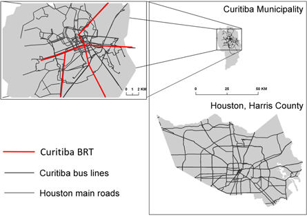
Houston exemplifies a city with low transport costs, corresponding to the paradigmatic example of the car-dependent city. Individual transport is cheap, and inhabitants can instead spend income on living space. This means that the city spreads further and as a consequence becomes less dense. Figure 7 shows the city structured by highways. There are more than 10 axes, which are connected by one small and one large ring highway. Such a city has already, due to an overall low density of 242 residents km−2 in the metropolitan area, a low UHI effect. Therefore, the reduction of CO2 emissions becomes the primary concern. We can see this in figure 5: for low transport costs, the point at which reducing the CO2 emissions stops being the main concern is only for a very high value of α. In other words, we have to value the reduction of the UHI effect very highly for it to become more important than the reduction of transport emissions. Consequently, such a low-density city would best be served with providing a high number of transport axes, as is illustrated in figure 6(a).
Figure 7. Bus system of Curitiba, and highway system of Houston. Both cities are structured by radial transport routes. In the case of Curitiba, there are five main bus rapid transit axes (not shown here); in the case of Houston there are 17 radial highways. Public transit allows for denser development along the transit axes, while car networks lead to wider dispersal of settlements.
Download figure:
Standard image High-resolution image
Curitiba has a slightly higher variance in elevation than Houston, ranging from approximately 850–975 m above sea level and averaging at roughly 935 m. An important local factor for the urban climate in Curitiba are the structural sectors imposed by the master plan guiding the development of the city. These corridors have an impact on ventilation and daylight accessibility. Consequently, challenges include thermal discomfort as well as possible effects on air quality (Krüger et al 2011, Krüger and Tamura 2015). Because of relatively cold temperatures in the city during winter months, the UHI at that time positively affects thermal well-being.
Curitiba exemplifies a city with a different urban design, oriented along BRT (figure 7) and resulting in higher transport costs in time for individual motorized modes. Even though it is the fourth richest city of Brazil, Curitiba has only one third of the per capita income of Houston, and hence inhabitants have less opportunity to purchase large housing space. Curitiba has a high population density of 4062 residents km−2 =40 residents ha−1.
In figure 7, the city centre is clearly discernible, together with four major axes (the two southern ones have been joined at the end). To reduce expenses, both in terms of time and money, individuals prioritize residential location that are attractive for commuting with public transit, in turn reinforcing a more compact urban form. As the travel distances are low in this high density city, the main concern quickly becomes the UHI effect. Figure 5 demonstrates that when transport costs are high, already a low value of α suffices to reduce the optimal number of axes. Therefore, such a city is best served with a low number of transport axes as illustrated in figure 6(b).
This comparison verifies that the main geometric properties of our model make sense. Curitiba has higher relative transport costs (given that per capita income is much lower), higher density, less area demand, and a smaller number of axes (5). In contrast, Houston has low transport costs, low population density, more area demand, and a higher number of transport axes (17). While Curitiba municipal policy makers intentionally designed its geometry with goals that are at least in alignment with climate change action, Houston did not. If Houston municipal policy makers prioritize climate change mitigation, they would charge automobile drivers. Curitiba is well advised to continue its policy of green area preservation to avoid increasing the risk of deadly urban heat waves.
Conclusion
Future-oriented urban planning needs to tackle the challenges of both climate mitigation and adaptation, goals that can be conflicting: more compact urban form reduces GHG emissions from transport, but increases urban heat stress, one of the deadliest consequences of climate change. Here we build a geometric model of urban design, informed by urban economics, that reveals a strategy to relax this trade-off: building star-like cities along linear transit axes. A higher number of axes will tend to mostly support climate mitigation, whereas a lower number of axes are conducive to reducing urban heat stress.
However, the underlying urban transport costs, both in time and monetary terms, remain a dominant factor in shaping urban form and resulting climate effects.
Our modelling results have several empirical correlates. (A) UHI is reduced by less compact, and more linear cities (Zhou et al 2017); (B) Green areas have a cooling effect radiating into surrounding built-up areas (Cheng et al 2015, Lin et al 2015); (C) urban economic models can replicate the distribution of cities with respect to population density and modal share as a function of transport costs (Newman and Kenworthy 1989, Creutzig 2014); (D) the effect of fuel prices on urban GHG emissions is empirically verified across a sample of 274 cities world-wide (Creutzig et al 2015). However, there is scope for empirical studies that use emerging big data on cities (Nangini et al 2019) to investigate the geometric features of cities and their relevance for climate mitigation and adaptation in more detail (Ilieva and McPhearson 2018, Creutzig et al 2019). In particular, combining remote sensing data with data on transport activities and temperatures at high spatial resolution for a number of cities that are comparable in terms of climate and socio-economic characteristics, will make it possible to disentangle the relevance of urban planning for climate change mitigation and adaptation. This will also help to overcome data limitations underlying this study, such as relying on a cooling decay function derived from observations from Shanghai only (Cheng et al 2015, Lin et al 2015).
Other social and environmental dimensions, such as air pollution and congestion are equally important in the design of cities. Air quality would profit from linear public transit axes, but high population density might be harmful, as it increases the fraction of pollutants breathed in (Lohrey and Creutzig 2016). Congestion might become worse, if considerable car traffic is routed via linear transit axes. Access to green spaces, a local quality of life dimension going beyond moderation of the UHI effect, however, would most likely improve. A complicated question involves consumption-based emissions. Residential living in dense inner-city areas in Helsinki has been associated with higher emissions from air travel (Heinonen et al 2013a). In the star-shaped city, dense residential living along the transit axes is associated with pedestrian access to green areas. Possibly, such access to green space counterfactually reduces air travel, a consideration that opens avenues for further research.
Our results are particularly important for rapidly urbanizing and developing cities, most of which are located in Asia and Africa (United Nations 2014), with more than 90% of urbanization-related GHG emissions until 2050 expected to come from these world regions (Creutzig et al 2015, 2016). Countries like China, India, Vietnam, and Nigeria differ in their specific urbanization dynamics and political environment, and hence there is no straightforward upscaling strategy for building star-shaped cities. However, a few tentative directions can be given.
First, many Asian cities are clogged with congestion and air pollution, and overmotorization is a key political issue. While climate change mitigation itself is not the main motivation, the local environmental concerns make alternative strategies to car and motorcycle centred urban mobility more attractive (Krzyżanowski et al 2005). Heat waves are a lethal danger to livelihoods in many African countries and South Asia (Mora et al 2017). Cities like Beijing are studied intensively both from the perspective of transport GHG emissions and UHI effect (Creutzig and He 2009, Miao et al 2009, Wang et al 2016). Hence, there is considerable attention and motivation to alleviate the urban climate challenges.
Second, any implementation strategy is likely to meet rapid urbanization dynamics that are hard to steer and control. It may be important to use price instruments, such as fuel taxes, to incentivise decentralized solutions that are more compatible to a public transit star-shaped city.
Third, the academic focus of both transport GHG emissions and UHI effect in Beijing may raise awareness of these issues especially in the Chinese capital, which in turn could facilitate upscaling of successful urban planning strategies. Importantly, Chinese cities and regions often follow the lead of successful example cities—a strategy dubbed the isomorphism of local development policies (Chien 2008), which has also been suggested to upscale low-carbon transport policies in China (Creutzig et al 2012). In fact, national policies already promote urban development that is consistent with climate mitigation and adaptation goals, and that could evolve into the design of star-shaped cities (Normile 2016). In India, cities grow more organically and unplanned. However, there is a growing and dynamic interest in providing policy frameworks that could facilitate the development of cities along transit axes (Ahluwalia et al 2014).
Fourth, Asia is at the forefront of development and financing models of transit-oriented development. In particular, Singapore and Tokyo have long-standing experience in financing the construction of high capacity mass transit axes via land value capture (Cervero 1998). This experience could also be leveraged for other rapidly developing cities in Asia and Africa.
In summary, this paper contributes to the joint negotiation of climate mitigation and adaptation concerns. It also proposes a new framework of analysis for sustainable cities, combining geometric and spatially explicit effects with urban economic modelling. We believe that this approach holds further potential for both relevant policy and intellectually stimulating research.
: Appendix: the UHI effect
Urban built environments heat up more than their rural surroundings, as building materials better absorb and store solar irradiation. Urban areas also often lack relevant cooling resulting from evaporation by vegetation. The local urban climate modifies the UHI in various ways, including through wind conditions, through street canyons that may channel wind (Oke 1988), but that may also provide shading (Johansson 2006), through mirror effects of glass facades, and through local vegetation (Susca and Gaffin 2011). In this paper, we focus on the geometric properties of urban form, as those play an important role in determining the strength of the UHI (Zhou et al 2017).
The UHI is a generic term. It is more accurately differentiated in terms of surface temperature and air temperature, with the former corresponding to the temperature of the surface, as measured by remote sensing, and the latter to the temperature of the air close to the ground, usually at a height of 2 m, as measured by local climate stations air temperature is likely to be of higher importance for climate impacts (including on human health). In this study, we base our evaluation of urban form effects on the surface UHI, as the underlying study of Zhou et al (2017) relies on remote sensing data. However, there is a high correlation between surface UHI and air UHI (Prihodko and Goward 1997), justifying the use of surface UHI for our modelling study.
The UHI can also be differentiated in terms of diurnal and seasonal nature. A global study of 419 cities has determined that the average annual daytime surface UHI is up to 2.1 °C higher than the average annual nighttime surface UHI (Peng et al 2012). A different study found for European cities a maximal saturation of the UHI in summer with a mean of 3 °C (Zhou et al 2013). Problematically, the terms urban and rural, which are used to define the UHI, denote a great variety of landscapes. This complicates the comparison of UHI studies since heterogeneous urban and rural situations are captured under the same term (Stewart and Oke 2012). In the case of a desert city like Phoenix, Arizona, studies have observed great potential for land system architecture to address the heterogeneous nature of the urban requirements (Connors et al 2013, Li et al 2017), suggesting that compact, regular green spaces (such as grass) can help reduce nighttime surface UHI, while irregular larger spaces can help reduce daytime surface UHI (Li et al 2017).
Modelling and simulation studies suggest that, e.g. for US American cities urban adaptation strategies are effective (Georgescu et al 2014, Ward et al 2016). Tree planting and urban greening belong to the key strategies mitigating urban heat stress (Fernandez Milan and Creutzig 2015). Green areas are commonly more abundant in leafy suburbs, compared to built-up inner cities. More compact cities tend to increase the UHI effect (Zhou et al 2017) and consequently worsen the impact of deadly heat waves (Mora et al 2017) (even if UHIs may often be of lower magnitude under warming conditions Scott et al 2018). While the UHI effect has positive effects in winter months in cities that have considerable heating demand, the impact of heat on health is emerging as one of the key and most harmful impacts of climate change (Gasparrini et al 2017). The concerns surrounding urban heat waves are only going to rise. Urbanization and more compact urban environments imply that a greater population is exposed to increased heat (Lemonsu et al 2015).
Footnotes
- 4
- 5
Curitiba's success story unfortunately is compromised by newly arising social exclusion, water pollution, and problematic public transport planning, partially enabled by the predominant narrative of its sustainable transport case, preventing institutional change (Martínez et al 2016).
- 6
This might suggest a neglect of the three-dimensional aspect of cities, yet compactness and density must not be confused here. While compactness measures, among other things, the ratio between built-up space and non-built-up space, density metrics measure the number of inhabitants or jobs per unit area; higher density is usually achieved by both reduced area per person, and higher buildings. Thus density metrics also translate into a three-dimensional profile of the city (Fujita 1989, Lemoy and Caruso 2018).
- 7