

Abstract
In June 2013, Uttarakhand experienced a hydro-meteorological disaster due to a 4 d extreme precipitation event of return period more than 100 years, claiming thousands of lives and causing enormous damage to infrastructure. Using the weather@home climate modelling system and its Half a degree Additional warming, Prognosis and Projected Impacts simulations, this study investigates the change in the return period of similar events in a 1.5 °C and 2 °C warmer world, compared to current and pre-industrial levels. We find that the likelihood of such extreme precipitation events will significantly increase under both future scenarios. We also estimate the change in extreme river flow at the Ganges; finding a considerable increase in the risk of flood events. Our results also suggest that until now, anthropogenic aerosols may have effectively counterbalanced the otherwise increased meteorological flood risk due to greenhouse gas (GHG) induced warming. Disentangling the response due to GHGs and aerosols is required to analyses the changes in future rainfall in the South Asia monsoon region. More research with other climate models is also necessary to make sure these results are robust.
Export citation and abstract BibTeX RIS

Original content from this work may be used under the terms of the Creative Commons Attribution 3.0 licence. Any further distribution of this work must maintain attribution to the author(s) and the title of the work, journal citation and DOI.
1. Introduction
Uttarakhand, situated in the north of India (figure 1(a)), is highly vulnerable to climate change due to its topography and socio-economic dependency on climate sensitive sectors such as agriculture, forest-based industry, tourism, animal husbandry and fisheries (Gosain et al 2015, UAPCC 2015). Changes in precipitation patterns, increases in temperature, reduced genetic biodiversity, glacier retreat, and the upward shift of agricultural cultivation zones have already been observed (UAPCC 2015). Historically, lighter, scattered rain showers were more frequent, which was beneficial for crops and recharging of aquifers (Jogesh et al 2016). In recent years, however, this pattern of lighter precipitation has increasingly been replaced by short, heavy downpours associated with increased runoff, soil erosion, and sometimes destructive floods and landslides (Ibid).

Figure 1. (a) Topography of India with zoom into the Uttarakhand region. (b) Daily mean precipitation variation in Uttarakhand during 1986–2015. The solid black line represents mean precipitation levels for 200 ensemble members of the model climatology. The purple, pink, and yellow lines show the precipitation field mean of 30 years of GPCC, CPC, and ERA-Interim precipitation, respectively. The grey, purple, pink and yellow envelopes show 10 to 90 percentiles of HadRM3P, GPCC, CPC, and ERA- Interim, respectively. (c) The QQ-plot with 50, 90, 95, 96, 97, 98, 99, 99.5 and 99.9th percentiles from the weather@home model ensemble and observational datasets. 4 d running means of rainfall for all four datasets are considered. (d) Time series of observed rainfall from 1900 to 2017. Note that HadRM3P and HadEX2 extremes are given in mm d−1, whereas CRU-TS, GPCC and CPC are given in mm/month.
Download figure:
Standard image High-resolution imageOne such extreme rainfall event occurred in mid-June 2013 (an extreme 4 d rainfall event), during which 370 mm d−1 of rain was recorded at Dehradun, which corresponds to 27% of the annual rainfall (Gosain et al 2015). Heavy rainfall caused a breach in a moraine dammed lake, leading to severe flooding that resulted in the loss of thousands of lives, and massive infrastructure damage that affected 4200 villages, 1636 roads, 144 bridges, and 19 hydropower plants (Das 2013, Rautela 2013, Dube et al 2014, Kala 2014, Gosain et al 2016). Reconstruction cost after the disaster is estimated to be almost 480 million pounds (Jogesh et al 2016).
Meteorologically, this rainfall event was caused by cold air intrusion of polar origin associated with an unusual incursion of a mid-latitudinal westerly trough, assisted by a low-pressure system over the Bay of Bengal (associated with a phase of strongly enhanced convection as part of the Madden–Julian Oscillation), and orographic lift at the Himalayas (Joseph et al 2014, Singh et al 2014, Ranalkar et al 2016). While these case-specific dynamic factors are always the major cause for extreme events, climate change tends to change the odds of such events occurring. Both, the mean as well as the shape of the distribution can change (Meehl et al 2000, Stott et al 2004, Pall et al 2011). According to Singh et al (2014), climate change has already made such extreme precipitation events more likely, when compared with pre-industrial conditions.
Here we estimate the change in return time of such extreme rainfall events under stabilized 1.5 °C and 2 °C scenarios, following the Half a degree Additional warming, Prognosis and Projected Impacts (HAPPI) protocol. This is in line with the temperature targets set out in the Paris Agreement. The event is defined as 4 d extreme precipitation with return period of about 100 years (Singh et al 2014). Using a large ensemble of climate simulations from weather@home, we quantify the risk ratios compared to current/actual and counterfactual/natural conditions (i.e. the climate we might be living in without human interference). By comparing actual with natural (pre-industrial) and greenhouse gas (GHG) only conditions (current world without anthropogenic aerosols), we can investigate the impact of aerosol pollution on monsoon rainfall in general, and the return period of extreme precipitation events in particular.
We complement our analysis with an estimate of future river flow for the Ganges at Haridwar, an important outlet point (78.11°E; 29.58°N) in Uttarakhand. Hence, in addition to the analysis on aerosol impacts, we combine information about the changing frequency of extreme rainfall events in the future with information on how these changes translate into the likelihood of future flood events. Each is vital for the development of disaster preparedness strategies, and for facilitating adaptation planning to minimize future damage from hydro-meteorological hazards. Lastly, we discuss the results in context of their uncertainties, together with an outline of remaining research gaps.
2. Methods
2.1. Model setup and observational data
We use results from a set of large ensemble, regional (HadRM3P) and global (HadAM3P) weather@home climate simulations (2nd generation; atmosphere-only). The advantage of the weather@home model setup is it allows for large ensemble simulations, enabling statistically robust analyses of extreme weather events, as demonstrated in many earlier attribution studies (e.g. Sippel et al 2015, Haustein et al 2016, Mitchell et al 2016, Schaller et al 2016). The regional model domain over the south Asian region has a spatial resolution of 0.44° × 0.44° (∼50 km on a rotated lat-lon grid; 19 vertical levels) and is nested within the global domain (Massey et al 2015, Guillod et al 2017). Each ensemble member is generated using initial (atmospheric) condition perturbation and/or different restart files.
Five climate scenarios are considered; all are derived from the weather@home simulations (using HadRM3P), but prescribed boundary conditions differ as follows (as per Massey et al 2015, Guillod et al 2017):
- 1.Natural/counterfactual scenario: matches with pre-industrial conditions as prescribed CO2 concentration is 280 ppm with no anthropogenic aerosols.
- 2.Actual climatology: prescribed with current conditions for all variables including CO2, aerosols concentration, SST, sea ice, land-use and land-cover.
- 3.GHG only scenario: same as actual, except prescribed concentrations of anthropogenic aerosols are zero.
- 4.HAPPI 1.5 °C: constrains global mean surface temperature (GMST) to 1.5 °C at the end of century (2091–2100). Representative Concentration Pathways 2.6 (RCP 2.6) is used to provide boundary conditions.
- 5.HAPPI 2 °C: constrains GMST to 2 °C at the end of century through a combination of RCP 2.6 and RCP 4.5 to prescribe the lower boundary conditions and the radiative forcing. Details of the generation of the prescribed SSTs, sea ice extent and radiative forcing data are provided in the supplementary information is available online: stacks.iop.org/ERL/14/044033/mmedia.
The HAPPI experimental setup is specifically designed to provide an ensemble of future climate that aims at setting a specific temperature, i.e. the radiative forcing is set accordingly, ensuring stabilized model scenarios (Mitchell et al 2017).
In our analysis, daily precipitation data from 98 simulations between 2006 and 2015 (2091–2100 in case of HAPPI) are examined for all five scenarios over a grid box that approximately covers the Uttarakhand region (77°–82° E and 28°–32° N). While the event in question occurred in early June during the onset of the monsoon, we investigate the change in risk over the entire rainy season (JJA) to increase the strength of the precipitation signal associated with anthropogenic aerosols. We have also compared the weather@home simulations with two other models MIROC5 and CAM4 for their actual, natural 1.5 °C and 2 °C scenarios (GHG only experiments are not available). However, these models are not used for the return period analysis for reasons discussed below.
To complement our analysis, total runoff derived from HadAM3P was routed by implementing the grid-based hydrological routing scheme as presented by Dadson et al (2011). This scheme is based on the discrete approximation to the 1D kinematic wave equation with lateral inflow and a Digital Terrain Model, constructed by using the Network Tracing Method (Olivera and Raina 2003) to delineate flow paths across river basins (Bell et al 2007). Since the scheme runs on 0.5° × 0.5° spatial resolution, the runoff was converted from the model grids accordingly. The runoff result should be used with caution as it is taken from a coarser GCM, HadAM3P, rather than its corresponding RCM, HadRM3P, due to lack of data availability. To find out how much caution is needed, we tested the skill of HadAM3P to simulate rainfall in the region of interest, by comparing the precipitation percentage changes and return period derived from HadAM3P and HadRM3P for the south Asian domain (figure S1). We also note that the river flow data could not be validated with observations as we were—despite uncounted attempts—unable to obtain the data from local authorities for the Ganges river. Therefore, ensemble means of CAM4 and NorESM1 is used to test the robustness of river flow data and conclusions are made accordingly. The robustness of HadAM3P's rainfall and river flow data is discussed in section 3.4.
We use the following observational datasets to evaluate the model and compare the attribution results. Global Precipitation Climatology Centre (GPCC): a gridded global (land only) daily rain gauge analysis collected from quality-controlled station data and provided by the German weather service (DWD) at a spatial resolution of 1.0° × 1.0° available since 1988 (Schneider et al 2008, Becker et al 2012). Climate Prediction Centre (CPC): NOAA's unified daily gauge-based precipitation analysis over land with spatial resolution 0.5° × 0.5° (Xie et al 2010). ERA-Interim: ECMWF generated daily gridded reanalysis precipitation product with a spatial resolution of ∼80 km (Dee et al 2011, ECMWF). HadEX2: the UK Met Office' gridded, station-based dataset of temperature and precipitation related climate extremes (Donat et al 2013). University of East Anglia's Climate Research Unit Time series (CRU)-TS v4.01: gridded monthly precipitation dataset with spatial resolution of 0.5° × 0.5° from 1900--2017 (Harris et al 2014).
3. Results and discussion
3.1. Model evaluation
To determine if weather@home HadRM3P regional model is suitable for our analysis, we evaluate the output against three daily observational datasets. Figure 1(b) shows the annual cycle of daily mean precipitation (mm d−1) averaged over the Uttarakhand grid box (77°–82° E and 28°–32° N; see figure 1(a)) for the weather@home actual climatology (200 ensemble member), ERA-Interim reanalysis, GPCC, and CPC datasets during the 1988–2015 period. In figure 1(c), the rainfall percentiles for summer (JJA) are plotted, whereas in figure 1(d) the time series of the monthly mean rainfall between 1900 and 2017 for different observational datasets are shown together with HadEX2. Note that HadEX2 and weather@home is given in units of mm d−1, while, CRU-TS, GPCC and CPC is in mm/month. Supplementary figure S2 shows the spatial differences between model, reanalysis, and observations.
All three daily observational datasets agree reasonably well with regard to magnitude and timing of the seasonal rainfall cycle (figures 1(b) and S2), with CPC being 30% dryer relative to other datasets during the onset of monsoon. Generally, rainfall is highest during the wet season (JJA) owing to the southwest monsoon, which contributes 77% of the state's annual rainfall (Gosain et al 2015). Interestingly, the weather@home model shows a secondary peak in September, which—while overestimated in strength and duration—is also present in the observations in early September. It is associated with the northeast monsoon, which only very weakly affects Northern India. HadRM3P reproduces the magnitude of the daily rainfall in Uttarakhand as far as GPCC and ERA-Interim is concerned. However, the model is out of phase during the onset (May/June) and retreat of the monsoon (September), which are approximately 30% wetter in the model compared to all observational estimates. In essence, the monsoon onset in the model is too early, possibly due to an overly sensitive triggering of orographic rainfall or influences from displaced extra-tropical atmospheric circulation features. Since we focus on the incremental change in return periods of extreme precipitation events between different future climate scenarios, we argue that it is valid to use the model without bias correction as these biases are likely caused by an inaccurate parameterization of the thermodynamic processes in the model, which leads to problems such as the overestimated orographic rainfall. Hence the problem is intrinsic to all scenario runs and scales with any given warming or climate scenario (see figure S3). Bias correction does not solve the problem, unless it is based on plausible physical considerations. For example, in Rimi et al (2018), a bias correction method based on a shifted time axis in the model is proposed to alleviate the early monsoon onset in a physically consistent way. But since we are not facing such issue in our analysis, the method would not remedy our biases.
The QQ-plot of 4 d running mean rainfall (figure 1(c)) shows that the model is in good agreement with GPCC and ERA-Interim, with the distribution of simulated rainfall closely tracking these datasets up to the 99th and 99.9th percentiles, respectively. As shown in figure 1(d), there is no long-term trend in the observations in the extremes (insignificant downward trend in the means), but there is a suspicious upward tick during the most recent years (after 2005) in all but the CRU-TS dataset. While this is by no means statistically significant, GHGs and anthropogenic aerosol might be playing significant role in intensifying monsoon cycle. Further discussion of this observation is provided in the results section. In general, there is a satisfactory level of agreement between the weather@home model and observational datasets for daily and accumulated 4 d running mean precipitation, with both the spatial and temporal variability of observed rainfall in the region well reproduced.
3.2. Change in spatial rainfall pattern
The results of the different modelling scenarios reveal that non-GHGs forcings such as change in anthropogenic aerosol emissions play significant roles in controlling future increases in rainfall over Uttarakhand. Firstly, our results reveal a change to substantially wetter conditions between the 1.5 °C versus actual results than between the 2 °C versus 1.5 °C results (see figures 2(a), (b), and S4). This apparent inconsistency can be explained by the reduction in aerosol emissions in the 1.5 °C and 2 °C simulations compared with actual conditions. (Note that both 1.5 °C and 2 °C scenarios are prescribed with almost 1/3rd of actual scenario's aerosols concentrations.) Evidence for this comes from the actual—GHG only results, where GHG forcing is kept the same for both model runs but aerosols are removed in the GHG only simulation, resulting in substantially drier conditions in the actual scenario (figure 2(d)). It provides strong evidence that the reduction in aerosols in the future warming scenarios (along with changes in non-GHGs factors) can largely be responsible for the substantially wetter conditions under 1.5 °C and 2 °C of warming. The non-GHGs effect also explains the apparent drying between the actual and natural simulations, where the GHG-induced wettening expected from the ∼1.0 °C of warming is overwhelmed by the drying impact of increased aerosol emissions (figures 2(c) and S4). The magnitude of the GHG-induced wettening effect is better revealed by the difference between the 1.5 °C and 2 °C simulations, where aerosols concentrations in both 1.5 °C and 2 °C scenarios are kept constant, and a temperature increase of 0.5 °C results in a wettening of ∼5% (figures 2(b) and S3: first row, third column).

Figure 2. Percentage change in ensemble mean precipitation during JJA in the HadRM3P regional model: (a) between 1.5 °C and actual, (b) between 2 °C and 1.5 °C, (c) between actual and natural scenario, (d) and between actual and GHG only. The black dots represent the regions where the difference between two scenarios are statistically significance at 95% confidence interval. Note that the region with the most intense changes (diagonal across each panel) is associated with the slopes of the Himalaya, where the model is particularly sensitive to any change in dynamics and thermodynamics.
Download figure:
Standard image High-resolution imageThe precipitation percentage changes derived from HadAM3P and HadRM3P are compared with CAM4 and MIROC5 for the south Asian domain (figure S3). The coarsely resolved CAM4 model (bottom row in figure S3; 2° spatial grid resolution) fails to capture the regional trends. While spatial resolution could be a contributing factor for the contrasting result (supported by the spatially very homogeneous percent changes in CAM4), factors such as limited sensitivity to changing aerosol concentrations are other key contributors. MIROC5 (third row in figure S3) is more sensitive to forcing changes, but does not agree well with HadRM3P, particularly for the actual versus natural case, which may be attributable to a reduced aerosol sensitivity of simulated rainfall in this model. Since its spatial resolution is equally limited and the ensemble size small, both, CAM4 and MIROC5 not considered for the return time analysis. We note that HadAM3P does also show discrepancies in case of 1.5 °C versus actual rainfall change (middle column in figure S3), which we attribute to an artefact in the global model version, namely an overestimation of drizzle when it should be completely dry. In dry regions, such as the Arabian Peninsula, the drizzle accumulates and leads to misleadingly high percent changes in response to changes in forcing. Because of the heterogeneous nature of the forcing (GHGs versus aerosols), HadAM3P and HadRM3P (which is less affected by the drizzle problem) show different percentage trends over very dry regions.
Our results confirm earlier studies that have investigated the inverse link between aerosols and the strength of the monsoon cycle (Ramanathan et al 2001, Lau et al 2006). For example, using a fingerprinting method, Bollasina et al 2014 found that once they remove aerosols in their model, the prolonged summertime drying over India in the late 20th century is replaced by widespread wettening. Physically, these changes result from altered latent and sensible heat fluxes at the surface due to reflection of incoming shortwave radiation by aerosol particles (Bindoff et al 2013). It is associated with evaporative cooling and a modified vertical temperature profile (Ban-Weiss et al 2011, Ban-Weiss et al 2012). Together with indirect aerosol effects such as cloud lifetime and cloud albedo effects, anthropogenic pollution acts to damp rainfall, which, in an attribution context, changes the risk assessment over time as fractional contributions from well-mixed GHGs and aerosols vary. Therefore, it is important to examine changing rainfall risks in context of anthropogenic aerosols and how an attribution analysis can be confounded when past and future forcing fingerprints are not considered (Bartlett et al 2018).
Without the incorporation of these past changes in aerosol and other non-GHGs forcing, the attribution analysis is bound to produce misleading results. This is not only applicable for a model analysis but also for an observation-based analysis. For example, should existing trends in rainfall (figure 1(d)) be extrapolated into the future, the missing (or slightly negative) long-term trend would suggest that the uptick after 2005 is due to natural variability. Instead, our GHG only results are suggestive of a possible, early emergence of the warming-induced GHG signal, as Asian aerosol emissions may decline in the near future due to efforts in combatting air pollution and massive investment in the renewables. According to Klimont et al (2013), the SO2 level in China have already peaked in 2005. While we do not know for certain, failing to disentangle the magnitude of the contribution from different anthropogenic forcing agents and, instead, implicitly assuming GHG induced warming alone is the sole driver of change, will almost certainly yield a misleading attribution outcome.
3.3. Estimation of return periods for rainfall extremes
In order to quantify the changing frequency of extreme 4 d rainfall events, in figure 3(a) we have plotted the return time for the seasonal maximum (JJA) 4 d (running) mean precipitation averaged over the Uttarakhand region. Most notably, there is only little difference in return times between actual and natural conditions, confirming the observation which show that the competing anthropogenic signals has not led to an increase in precipitation return time in this region so far. We find no drying for the seasonal maximum as opposed to a drying trend in the mean (figures 2(c) and S5). In contrast, return times for the 1.5 °C scenario have significantly decreased relative to actual conditions, in broad agreement with the change in the mean (figures 2(a) and S5). The return times for the GHG only simulations are just above those of the 1.5 °C scenario, providing further evidence that the suppressed rainfall under current conditions is mostly due to non-GHGs forcing, particularly anthropogenic aerosols. In fact, the GHG only simulations in which anthropogenic aerosols are absent, suggest that extreme rainfall is likely to become more frequent in the future if aerosols concentration plummets due the implementation of air quality control measures. It is highly likely that aerosols levels will eventually come down regardless of the time it takes; thus, we may as well refer to the aerosol drying effect as committed future wettening effect.
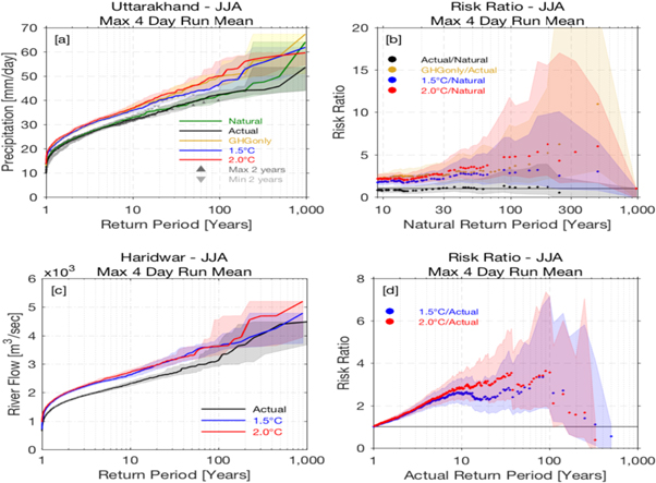
Figure 3. Return periods (a) and risk ratio (b) for maximum seasonal 4 d running mean precipitation and 4 d river flow and its associated risk ratio (c) and (d) during JJA in five (three for river flow) different scenarios. Shaded envelopes represent the 5–95th percentile rainfall ranges for each scenario, estimated using bootstrapping with 1000 realizations. Grey triangular bands in (a) refer to the same rainfall quantity but subsampled for the two years of maximum (upper diamond) and minimum (upper diamond) summer mean precipitation over Uttarakhand based on the actual model ensemble.
Download figure:
Standard image High-resolution image
The grey series of return times in figure 3(a) is a subsample of the actual ensemble, constructed using the two years (out of the 10 years between 2006 and 2015) of maximum and minimum monsoon mean precipitation over Uttarakhand (upper and lower triangles). It illustrates the degree of natural variability in comparison to the forced signal. Similarly, figure S5 visually underscores the change in strength of the monsoon cycle between the different scenarios in comparison to the absolute rainfall amount. Interestingly, despite comprising one of the strongest La Niña's on record (2011) and at least one moderate El Niño (2010) the signal-to-noise ratio is rather high. The forced signal under 1.5 °C and 2 °C conditions exceeds natural variability by a considerable and significant margin. While these changes appear to be relatively small in comparison, it is the extremes that cause the majority of the hydro-meteorological damage. Even a slightly increased frequency of occurrence can have enormous impacts on agricultural production, water resources management and the overall economy of the state as exemplified by the 2013 extreme rainfall event.
According to simulated change in return time for an extreme event 4 d rainfall event, a 1-in-100-year event (uncertainty range: 1-in-51-year to 1-in-192-year) for the actual world scenario is projected to be a 1-in-39-year event in the 1.5 °C warmer world (uncertainty range: 1-in-25-year to 1-in-61-year) and a 1-in-23-year event (uncertainty range: 1-in-16-year to 1-in-33-year) in the 2 °C warmer world. Risk ratio graph (figure 3(b)) implies that an event similar to the June 2013 event is projected to increase by a factor of 2.7 (Uncertainty range: 1–7) and 4.8 (Uncertainty range: 2–11) in 1.5 °C and 2 °C warmer world scenarios when compared with natural conditions, respectively. However, we caution that the uncertainty for return periods >100 years is very large due to the comparably low number of model simulations.
In addition to the 4 d seasonal maximum, we have also estimated the return time for 5, 15, and 30 d seasonal maxima as these are time periods more relevant for river discharge and associated river flow (see figures S6, S7 and table S1). In general, we find that there is a significant difference in the return period for longer rainfall events compared to the 4 d seasonal maxima. In particular, we find that the influence of non-GHG forcing including aerosol is even stronger for longer (extreme) rainfall intervals. Our results suggest that the increase in rainfall due to lower level of aerosol in the future scenarios is what drives the bulk of the change towards 1.5 °C and 2 °C. In fact, the frequency of flash floods (1–2 d extremes) as well as river flooding (5–30 d extremes) are likely to substantially increase. Provided that even a slight increase in temperature increases the risk of extreme events already, it is vital to pursue efforts to limit global warming as outlined in the Paris Agreement. Continued warming is likely to have serious and irreversible impacts on extreme rainfall events in Uttarakhand.
3.4. Estimation of return periods for river flow
To illustrate the change in river flow, in figure 3(c) the results for the Haridwar station at the Ganges river in the Uttarakhand region is shown for 4 d seasonal maximum flows under current, 1.5 °C and 2 °C conditions. Since we only have daily runoff data from the global weather@home model, we first estimate the impact of change in resolution for precipitation between HadAM3P and HadRM3P (see figure S1). We find that the global model underestimates JJA rainfall by ∼50%, which in turn causes runoff to be underestimated by a similar amount. As a consequence, the river flow will be biased low as well. Using two of the other HAPPI models that provide daily runoff (CAM4 and NorESM1) we compare their associated river flows at Haridwar (Ganges) with HadAM3P. As shown in figures S8 and S9, the annual cycle as well as the annual mean precipitation is underestimated by a factor of 4 to 5 in the HadAM3P.
Interestingly, both CAM4 and NorESM1 simulate much higher and more realistic rainfall rates across tropical latitudes compared with HadAM3P. While CAM4 and NorESM1 do have a higher spatial resolution, it is most likely their more advanced convective parameterization schemes that lead to a much better model performance with regard to precipitation and runoff. Accordingly, the calculated river flow is vastly different. It is important to note, however, that HadRM3P alleviates most of this bias; hence we are confident that in future studies (when we runoff from HadRM3P will be available) the river flow bias will largely disappear. Given that the results are robust with regard to the risk ratios in the global and regional case across the available range of possible return times (see figure S1), we refrain from scaling the river flow results in this study, but we will do so in the future where observational river flow data are available. We consider this analysis a proof of concept with the aim to demonstrate that we can make qualitative assessments of river flow.
In quantitative terms, we find that the return period of the Ganges 4 d seasonal maximum flow at Haridwar has decreased by ∼80% for a 1-in-100-year event (risk ratio is 3.7 with uncertainty range 2–7) in both 1.5 °C and 2 °C scenarios with respect to actual scenario. Given that river flow is more controlled by longer extreme rainfall events, the fact that risk ratios for 15 or 30 d mean precipitation (figures S6 and S7) resemble that of the river flow for both warming scenarios can be remarkable.
Despite the caveats and uncertainties, this significant and rather drastic increase in risk by a factor of ∼4 for extreme 4 d flood events between current conditions and the soon to be reached level of 1.5 °C warming, indicates that there is a looming danger for considerably more frequent severe flooding, irrespective of the anticipated additional warming as alluded to above. Given the peculiar uptick in rainfall intensity (figure 1(d)), the Uttarakhand flood in June 2013 might have been a harbinger for what is to come, with potentially worrisome consequences for vulnerable regions such as Uttarakhand.
4. Conclusions
Using model simulations carried out within the framework of the HAPPI experiment, we find that in a 1.5 °C warmer world (where aerosol levels are 1/3rd of actual scenario) the combined effect of continued GHG warming and aerosol reduction leads to a strong increase in the frequency of occurrence of extreme precipitation events. The smaller increase in precipitation between 1.5 °C--2 °C (compared to the change between the current level of 0.9 °C--1.5 °C) indicates that non-GHGs forcing can be a very potent driver for changes in the hydrological cycle over the region, leading to a high degree of nonlinearity between the forcing scenarios. As such, current conditions (or the change between current and 1.5 °C warmer conditions) are a very poor predictor for future conditions. Therefore, it is of vital importance to separate the two major anthropogenic forcing factors (GHGs and aerosols) and recognize that there is a considerable degree of committed/irreversible change in the likelihood of extreme rainfall events.
We have also investigated that change in risk in river flow at Haridwar in the Ganges and found that the river flow is expected to increase drastically in between now and a 1.5 °C warmer world (∼80%). The increase in risk is higher than that of short-duration precipitation, which is likely related to the stronger increase upstream of the Ganges catchment area compared to the rainfall change in the Uttarakhand region only. In combination with the missing trend in more severe precipitation until now, we argue that the counterbalancing drying effect of non-GHGs forcing, specifically aerosols may lead to a false sense of security, which—despite considerable caveats—does not appear to be justified.
To sum up, the return time results indicate that the precipitation levels in a 1.5 °C and 2 °C warmer world are significantly higher than under current conditions. Given that the monsoon season is already wet in the Uttarakhand region, further increases in rainfall infer more frequent rainfall-related disasters. It is therefore of primary importance to explore possible adaptation and mitigation measures to plan for a future in which extreme precipitation and flood events are more common. It is, therefore, desirable to accelerate the transitioning to a low carbon economy so that we can limit the temperature increase to 1.5 °C as outlined in the Paris Agreement. Further studies with higher resolution models and varying physical parameters associated with convective activity are needed to systematic model biases and to identify regions and/or scenarios of greatest impact.
Acknowledgments
This work has been partly funded by the EPSRC Global Challenges Research Fund (EP/R512850/1). The authors are grateful to Oxford University Centre for the Environment for supporting our research project. (All weather@home and HAPPI data are available online: http://portal.nersc.gov/c20c/data.html.) Other information can be obtained by emailing the corresponding author.