

Abstract
Machine learning promises to advance analysis of the social and ecological impacts of forest and other natural resource policies around the world. However, realizing this promise requires addressing a number of challenges characteristic of the forest sector. Forests are complex social-ecological systems (SESs) with myriad interactions and feedbacks potentially linked to policy impacts. This complexity makes it hard for machine learning methods to distinguish between significant causal relationships and random fluctuations due to noise. In this context, SES frameworks together with quasi-experimental impact evaluation approaches can facilitate the use of machine learning by providing guidance on the choice of variables while reducing bias in estimated effects. Here we combine an SES framework, optimal matching, and Causal Tree-based algorithms to examine causal impacts of two community forest management policies (forest cooperatives and joint state-community partnerships) on vegetation growth in the Indian Himalaya. We find that neither policy had a major impact on average, but there was important heterogeneity in effects conditional on local contextual conditions. For joint forest management, a set of biophysical and climate factors shaped differential policy impacts across the study region. By contrast, cooperative forest management performed much better in locations where existing grazing-based livelihoods were safeguarded. Stronger local institutions and secure tenure under cooperative management explain the difference in outcomes between the two policies. Despite their potential, machine learning approaches do have limitations, including absence of valid precision estimates for heterogeneity estimates and issues of estimate stability. Therefore, they should be viewed as a complement to impact evaluation approaches that, among other potential uses, can uncover key drivers of heterogeneity and generate new questions and hypotheses to improve knowledge and policy relating to forest and other natural resource governance challenges.
Export citation and abstract BibTeX RIS

Original content from this work may be used under the terms of the Creative Commons Attribution 3.0 licence. Any further distribution of this work must maintain attribution to the author(s) and the title of the work, journal citation and DOI.
1. Introduction
Community-based forest management relies on the involvement of local communities in resource governance to improve social and ecological outcomes. Governments and other funders have invested millions of dollars to promote community participation in forest management [1, 2]. Initiatives include formation of local community institutions and downward transfer of forest resource tenure to enhance and protect forest resources [3, 4]. Evidence of the success of such community-based interventions is mixed and highly heterogeneous [2, 3, 5–7]. Understanding how forest management policies perform, and which social and ecological contexts are more conducive for success over the long term is critical to enhancing their effectiveness [8]. Recent machine learning (ML) approaches hold particular promise for building knowledge in this domain and on natural resource policy more generally.
ML approaches rely on data to understand generalizable patterns. Unlike commonly used econometric impact evaluation approaches, ML flexibly adapts algorithms based on data to make predictions that can uncover complex structures in the data that are not specified a priori [9, 10]. The ability of ML to use data to make efficient decisions regarding bias-variance trade-offs and allow high degree of interactivity among variables enables such approaches to predict outcomes in a reliable, repeatable manner [11]. ML approaches perform especially well in finding functional forms that work well out-of-sample [9].
These attributes mean that ML approaches have considerable potential for use in conservation and natural resource policy. For example, ML can enable translation of satellite data to ecological and social outcome measures by extracting and scaling meaningful signals to a broader study area based on a few sample locations [10, 12]. This capacity holds particular value for policy evaluation in areas where reliable socio-economic data are limited [12, 13]. ML methods can also complement theory-driven econometric strategies by illuminating different factors shaping outcomes of interest and generating predictions for further testing [14–16]. Because ML approaches can identify variation in impacts that standard interaction effects fail to detect [17], they may have special relevance to environmental and natural resource policy where complex interaction among social and ecological factors is often a defining feature. ML approaches such as decision trees [18], random forests [15] and ensemble methods [19] have been used to assess such heterogeneity. Finally, given the capacity of ML approaches to uncover complex, sometimes unanticipated patterns in data, they can help suggest theory about causal mechanisms [11] and provide information to improve intervention targeting [17].
ML methods are not a panacea, however. They must be used carefully, with recognition of their limitations and advantages compared to other approaches. For example, the predictive functions used in ML can pose a challenge for causal interpretation [20–22]. Further, estimates derived from ML models do not equate to parameter estimates obtained in regression or other econometric methods and the absence of standard errors limit inference after model selection. Interpreting the estimated parameters from ML methods as indicative of the underlying structure of the data is naïve and requires careful attention [9]. For these reasons, ML should be considered a complement to rather than a replacement for theory-based econometric approaches.
To date, ML approaches have seen little application in relation to forest and natural resource policy. Limited data availability, the complexity of many social-ecological contexts, and uncertainty about the potential of ML help explain why such approaches have not found significant uptake in this domain. Forest programs do not usually yield 'big data' and lack granular-level data on features and related outcomes, restricting ability to use ML [23]. The social-ecological systems (SESs) where forest programs are implemented are often complex, challenging efforts to capture relevant variables and feedbacks among them linked with policy outcomes [24–26]. Given this complexity, ML algorithms may also struggle to distinguish between significant patterns and random fluctuations due to correlated noise.
Our goal in this paper is to demonstrate that ML approaches can make a valuable contribution to understanding natural resource policy and that it is increasingly possible to use them in this field. We integrate a ML approach with SES theories and econometric methods to analyze the social-ecological impacts of two different community forest management policies, cooperative forest management (CFM) and joint forest management (JFM), in the Indian Himalaya. In particular, we use Causal Tree (CT) and Causal Forest (CF) decision-tree algorithms [18] in combination with an SES framework and optimal matching to estimate the heterogeneous causal impacts of these policies and identify key factors associated with observed ecological outcomes. Our approach has wide potential to be applied in diverse settings around the world to build knowledge on the causal pathways and impacts of forest and other natural resource policies.
2. Data and methods
Data in our study derive from 202 Forest Management Regions (FMRs) in Kangra District, Himachal Pradesh, India (figure 1) over a period of 14 years (2002–2016). The treatment group includes all FMRs that were under CFM and JFM between 2002 and 2006. The CFM treatment group consists of 15 FMRs where CFM was implemented while the JFM treatment group includes the 38 FMRs where JFM was implemented.

Figure 1. Community forest management regimes in the study area.
Download figure:
Standard image High-resolution imageBuilding from institutions put in place under the Kangra Forest Cooperative Societies Scheme starting in the 1940s [27, 28], the state government began to reinvest in CFM in Kangra district from 2002–2005 to support sustainable forest management. This investment included financial and technical support to village-level forest cooperative bodies and organizational support to the formation of a federation of forest cooperatives mobilized by a local NGO. Investment started in 2002 and each participating FMR had received early support by 2005. For this reason, we use data from 2002 to 2005 as a baseline in our impact assessment.
JFM (a Forest Development Agency program funded by the national government) was the flagship community participatory initiative for forests in India starting in the 1990s [29–31]. In the early 2000s, JFM interventions were begun in several of the study FMRs to involve communities in forest regeneration and protection. This program supported local participation in afforestation programs to enhance tree cover and boost local livelihoods. Communities were organized into JFM committees to raise and protect plantations on public lands [29, 31]. A key difference between this program and CFM is that it did not allocate forest property rights to communities or the right to derive revenue from forest resources claimed by the state. The baseline for this program is the same as that for CFM.
We expect CFM regimes to improve long-term ecological outcomes at the FMR level through collective action due to the institutional strength and tenure rights of the forest cooperatives. Cooperative members may supply labor, resources, and information to other members and forest officials, and may help engender sustainable forest resource use through mutual monitoring and enforcement of rules [32, 33]. On the other hand, the transient nature of village institutions and absence of secure forest tenure over forests under JFM leads us to hypothesize that this intervention will have less favorable impact on long-term ecological outcomes.
The outcomes of these two policies are measured using a Normalized Difference Vegetation Index (NDVI), a proxy for vegetation growth [34]. We calculated NDVI as an average value of NDVI (mean, annual) for FMRs for the period between 2011 and 2016. We expect a temporal lag of 5–9 years between the start of CFM and JFM (during the 2002–2005 period) and their ecological outcomes (e.g. improved vegetation growth). The reason is that planted seedlings or protected natural regenerated areas typically require at least five years to yield substantial improvement in NDVI values (i.e. increased tree cover). Because FMRs in the study area do not usually have very high NDVI values, NDVI saturation is unlikely to be an issue in our analysis.
2.1. Variable selection
To analyze the effects of these two forestry policies, we first identified a set of 28 relevant SES variables and associated indicators (tables 1 and S1 are available online at stacks.iop.org/ERL/14/024008/mmedia) based on SES and common property research [24–26, 35] and our in-depth knowledge of the study context. Indicator data derive from publicly available secondary social and spatial datasets (see references in table S1). We included this range of variables to allow our ML approach to choose those with the highest importance in predicting the heterogeneous impacts of the two forestry polices. Our approach enabled us to explore potential interaction effects among variables in order to predict effects for specific FMRs rather than only an average treatment effect for the entire population under study.
Table 1. Social-ecological system variables related to long-term ecological outcomes (Normalized Difference Vegetation Index, mean annual) in forest management regions (FMRs) in Kangra District, Himachal Pradesh, India.
| Variable | Indicators | All FMRs (n = 202) | CFM FMRs (n = 15) | JFM FMRs (n = 38) |
|---|---|---|---|---|
| Sub-system 1: actors | ||||
| 1. Users | Number of households | 1080 | 1987 | 764 |
| Number of villages | 13 | 16 | 9 | |
| Number of cultivators | 317 | 469 | 239 | |
| Number of marginal people | 1067 | 2175 | 765 | |
| 2. Socioeconomic conditions | Number of literate people | 3685 | 6930 | 2560 |
| Number of unemployed people | 1011 | 1537 | 823 | |
| Economic activity (1–63, values) | 5.05 | 7.15 | 3.62 | |
| Road density (km/km2) | 1.11 | 1.12 | 0.95 | |
| 3. Importance of resource | Number of smallholdings | 921 | 785 | 1083 |
| Sub-system 2: governance | ||||
| 4. State afforestation programs | Area planted (ha) | 80.48 | 6.45 | 5.09 |
| Broadleaf sp. planted (%) | 38.36 | 42.76 | 38.14 | |
| Number of nurseries | 0.27 | 0.33 | 0.37 | |
| Sub-systems 3 and 4: resource units and resource system | ||||
| 5. Mobile animals | Number of grazing animals | 4970 | 5528 | 5358 |
| 6. Size of resource system | Forest beat area (ha) | 1756.14 | 2487.08 | 1742.02 |
| Tree cover (ha) | 1037.7 | 1014.58 | 1100.83 | |
| Crop acreage (ha) | 41.44 | 58.56 | 34.66 | |
| Grass acreage (ha) | 16.47 | 11.85 | 17.83 | |
| Bare land acreage (ha) | 0.97 | 0.06 | 1.9 | |
| 7. System productivity | Soil depth (cm) | 95.1 | 100 | 88.16 |
| Total carbon (Kg C m−2) | 7.58 | 6.87 | 7.92 | |
| Total organic carbon (% weight) | 1.36 | 1.16 | 1.48 | |
| Available soil water capacity (mm) | 99.58 | 123.33 | 80.92 | |
| Baseline vegetation/NDVI (−1 to 1) | 0.5 | 0.49 | 0.5 | |
| 8. Location | Altitude (m) | 874.79 | 658.79 | 1099.6 |
| Interactions (I) | ||||
| 9. Conflict among users | Number of forest fires | 1.96 | 0.24 | 0.1 |
| Outcomes (O) | ||||
| 10. Ecological performance | NDVI (−1 to 1) | 0.5 | 0.51 | 0.53 |
| Related ecosystems (ECO) | ||||
| 11. Climatic factors | Temperature (degree Celsius) | 18.26 | 19.68 | 16.15 |
| Precipitation (mm) | 77.09 | 78 | 76.65 | |
| Land surface temperature (Kelvin) | 297.05 | 298.5 | 295.6 | |
Note: all values are averages for the full study period (2002–2016); CFM, cooperative forest management; JFM, joint forest management. Further details on these variables and their sources can be found in the supplementary information, table S1.
2.2. CT estimator
CT is a decision tree–based approach derived from ML methods to recursively partition units under study into smaller groups so as to identify heterogeneous treatment effects [18]. The method builds on CART (Classification and Regression Trees) with the difference that CT focuses on estimating conditional average treatment effects (CATE) rather than predicting outcomes. CT is useful in cases where number of attributes exceeds the number of units studied and in cases where the functional forms of relationships between the attributes and the treatment effects are not known [18].
We used an 'honest' approach [18] in which the CT algorithm does not use the same information for selection of the model structure as for estimation given this model structure. To do so, the sample is split into two parts, one part for constructing the tree (including the cross-validation) and a second part for estimating treatment effects within leaves of the tree. This method uses unbiased estimates of the mean squared error as the criterion to evaluate the causal effect of the treatment. The honest approach is used to guarantee consistency or asymptotic (large sample) normality of predictions [18].
CT assumes random assignment to treatment group. In observational studies like ours, this assumption is hard to fulfill. Thus, we used optimal matching to create treatment and control groups to reduce possible bias from simple comparisons of treated and control units. We then use the matched treated and control groups in a CT algorithm (in R) to calculate the heterogeneous causal effects of CFM and JFM interventions.
The tuning parameter for the CT function is to have a minimum number of treated and control observations per leaf to calculate treatment effect within each leaf. In the splitting function, there is a restriction on the set of potential split points. Later in the splitting process the covariate values within each leaf and each treatment group are rescaled to ensure that the same number of treatment and control observations are moved from the right leaf to the left leaf when moving from one potential split point to the next. The causal function uses a minimum of five cross-validation samples as another tuning parameter to produce the best-fitted predictive model of heterogeneous treatment effects [18].
Our CT specification uses an honest splitting rule with fit as a cross-validation method. We used 5-fold cross-validation with a discrete splitting option. The treatment probability is set as propensity = 0.5 for the CT splitting rule. Table S2 presents complexity parameters and normalized cross-validation error. For tree selection we chose a complexity parameter corresponding to the minimum cross-validation error. Thereafter we used the prune () function to trim the selected tree by removing the branches using features with low importance. Pruning increased the predictive performance of the tree by reducing overfitting [36].
We used CF to estimate standard errors associated with causal effects, particularly the CATE for the whole region and treated FMRs (CATT, CATE on the treated) [15, 37]. This approach provides more stable estimates compared to CT, even as CT algorithm results are comparatively easier to interpret from a policy perspective [15, 37]. We also used the CF algorithm (based on growing of 5000 CTs) to validate predictors of the heterogeneous treatment effects identified as most important by the CT algorithm [15, 37].
2.3. Optimal matching
We used optimal matching [38] to create a matched control group for the treated FMRs in our analysis. This matching-based identification strategy is a quasi-experimental methodology to evaluate various programs and policies [38–40]. We chose optimal matching due to its ability to identify the same sets of control units for the overall matched treated units with the smallest average absolute distance across all matched pairs. This approach was also preferable due to the absence of a large number of appropriate controls for our treated units [41].
We matched on a subset of the 28 variables in our SES framework most likely to influence the uptake of studied policies and vegetation outcomes in FMRs (table S3). This selection was based on previous research and our contextual knowledge of the study region [31, 42]. We expect that our chosen set of factors largely capture the background differences between control and treatment groups and effectively serve as proxies for the effects of potential moderators/variables that were not included. We then used the chosen variables for matching treatment and control groups to obtain a counterfactual for the treated FMRs.
Optimal matching created matched control groups for FMRs under CFM and JFM interventions from the available pool of potential control FMRs in Kangra District. For the group of 15 CFM-treated FMRs, optimal matching created a control group of 75 FMRs out of 187 available control FMRs (out of the 202 total FMRs). In the case of JFM, for the treated group of 38 FMRs, optimal matching created a control group of 152 FMRs out of 164 available control FMRs. The covariate balance is given in the supplementary information (<0.25 standardized t diff as threshold; see table S3).
3. Results and discussion
Neither CFM nor JFM appear to have had large overall impacts on long-term vegetation growth (NDVI, 2011–2016) (figure 2, table 2). Results using the CT method show that the magnitude of the average treatment effects of both policies was very low in the region (CFM: −0.000006; JFM: 0.004). These findings are further corroborated by the CF algorithm, which also shows very low and non-significant CATE for both policies (table 2).
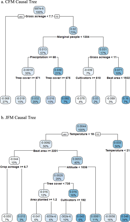
Figure 2. Causal Tree: heterogeneous causal impacts of (a) cooperative forest management (CFM) and (b) joint forest management (JFM).
Download figure:
Standard image High-resolution image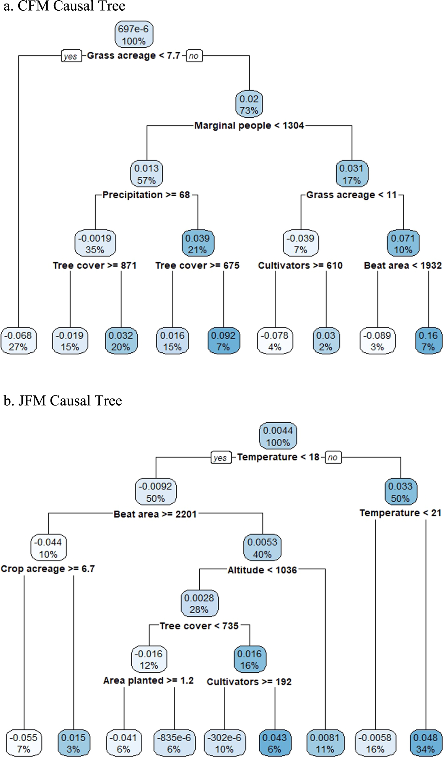
Table 2. Conditional average treatment impacts of cooperative forest management (CFM) and joint forest management (JFM) on NDVI.
| Forest policy | Conditional average treatment effect for the whole region (CATE) | Conditional average treatment effect on treated FMRs (CATT) |
|---|---|---|
| CFM | 0.001 (0.004) | 0.0004 (0.005) |
| JFM | 0.0009 (0.002) | 0.0004 (0.003) |
Note: results based on the Causal Forest (CF) algorithm. CF specification: number of trees = 5000; honesty = false; number of fit trees in each 'mini forest' in tuning model = 200. Standard errors in brackets.
These results mask important heterogeneity, however. The next two sections therefore describe the heterogeneous causal effects of CFM and JFM using CT and elicit the contextual conditions that facilitate favorable causal impacts for both policies.
3.1. Heterogeneous causal effects of CFM
CFM results were heterogeneous and varied according to different contextual social and ecological factors (figure 2(a), table 3). Grass acreage was the most important predictor. Variable grass acreage in FMRs initiated the first split of the CT to obtain two sub-groups: one with FMRs where CFM led to increases in vegetation growth and the other where CFM had a negative impact on vegetation growth. FMRs with higher values of grass acreage (=>7.7 Hectares) showed a positive impact on vegetation growth (0.02 increase in NDVI; observations 73%) whereas FMRs with lower grass acreage (<7.7 hectares; observations 27%) showed a sizeable negative impact on vegetation growth (−0.07). The number of marginal people was the second most important predictor, with the causal impact of CFM on vegetation growth about three times more in FMRs with a higher number of marginal people (>1304) compared to the FMRs with less. The CT we selected has a complexity parameter corresponding to minimum cross-validation error to maximize predictive power without 'overfitting' (size of tree = 15; table S2(a), figure S1) [18].
Table 3. Heterogeneous causal impacts of cooperative forest management (CFM) on NDVI.
| Causal pathways | Predictor I | Predictor II | Predictor III | Predictor IV | Conditional average treatment effects |
|---|---|---|---|---|---|
| a. Conditions associated with positive impacts | |||||
| I | Grass acreage (> = 7.7 ha)a | 0.02 | |||
| II | Grass acreage (> = 7.7 ha) | Number of marginal peopleb > = 1304c | 0.03 | ||
| III | Grass acreage (> = 7.7 ha) | Number of marginal people > = 1304 | Grass acreage (> = 11 ha) | 0.07 | |
| IV | Grass acreage (> = 7.7 ha) | Number of marginal people > = 1304 | Grass acreage (> = 11 ha) | Forest beat area > = 1932 had | 0.16 |
| b. Conditions associated with negative impacts | |||||
| I | Grass acreage (<7.7 ha) | −0.07 | |||
| II | Grass acreage (<11 ha) | Number of cultivators > = 610e | −0.08 | ||
Note: predictors I, II, III, IV are ranked as per their importance in achieving the best performance predictive CT algorithm (with minimum cross-validation error and optimal level of complexity). aValue of 7.7 ha is 17th percentile on the total distribution of grass acreage in the study area (202 FMRs). bNumber of marginal people represents individuals belonging to the Scheduled Caste category. This official category is designated by the government as historically disadvantaged and socially and economically marginal for affirmative action. cValue of 1304 is 74th percentile on the total distribution of marginal population in the study area. dValue of 1932 ha is 71th percentile on the total distribution of areas of forest beats in the study area. eValue of 610 is 87th percentile on the total distribution of number of cultivators (farmers) in the study area.
Under CFM, forest cooperatives have durable tenure over their forests. Secure tenure is expected to improve local livelihoods due to improved access to biomass (e.g. for energy needs) and lower cost of sustainable forest management due to higher local participation in the protection and management of forests [43–45]. Moreover, durability of institutional tenure has been shown to be positively related to improved forest condition [46].
Our results confirm these prior findings and show that the impact of secure tenure was conditional on local social and ecological contextual factors (table 3(a)). CFM led to a positive impact on vegetation growth in the medium to long term (5–9 years after intervention), especially when members of the cooperatives had greater access to grazing areas (>7.7 ha, first causal pathway, 18th–100th percentile). These grazing areas provide members of community organizations with a regular source of income through grass auctions and grazing resources to support local livestock-based livelihoods.
We find that CFM led to increases in NDVI even in FMRs with a higher number of marginal people (causal pathways II–IV, 74th–100th percentile). Marginalized populations are expected to have higher forest dependence due to their heavy reliance on local forest resources for subsistence needs such as grazing and collection of fuelwood, fodder, and small timber. However, CFM appears to moderate such forest dependence, leading to positive long-term vegetation growth as found in other studies in the region [27, 28]. Finally, we find that the ecological performance of CFMs was much better in the context of FMRs with larger grass acreage, a marginalized population, and larger overall area (71st–100th percentile) (causal pathway IV). This finding is likely due to better availability of resources as FMR size increases, which may help disperse local user pressure on forests.
Several contextual social and ecological factors were not conducive to CFM success (table 3(b)). Despite the presence of strong forest tenure, low availability of grazing lands in the FMRs (1st–17th percentile) can reverse the positive effects of tenure over long-term social and ecological outcome trajectories. This result indicates that local participation in forest improvement and protection efforts is unlikely in the absence of sufficient grazing lands. This unfavorable impact of CFM on vegetation growth further intensifies with increasing numbers of cultivators (farmers). More cultivators likely means greater reliance on forests for subsistence needs and, in turn, increased pressures on forests resulting in decreased vegetation growth [32, 42].
3.2. Heterogeneous causal effects of JFM
The social and ecological contexts conducive to long-term vegetation growth were different in JFM than CFM. Temperature was the most important variable shaping the heterogeneous impacts of JFM in the study region (figure 2(b), table 4). JFM led to higher and positive impact on vegetation growth in FMRs that experienced 18 °C or more temperature (0.03; observations 50%) compared to FMRs with less than 18 °C (−0.009; observations 50%). However, out of 50% FMR observations with temperature less than 18 °C, the impact of JFM on vegetation growth varied with area of the FMR. FMRs with area less than 2201 hectares experienced positive impact of JFM compared to FMRs with area greater than or equal to 2201 hectares. Further splitting of the data explains additional treatment heterogeneity conditional on important predictors. As for our CFM analysis, we selected CT with a complexity parameter corresponding to minimum cross-validation error (size of tree = 9; table S2(b) and figure S2) [18].
Table 4. Heterogeneous causal impacts of joint forest management (JFM) on NDVI.
| Causal pathways | Predictor I | Predictor II | Predictor III | Predictor IV | Conditional average treatment effects (ATT) |
|---|---|---|---|---|---|
| a. Conditions associated with positive impacts | |||||
| I | Temperature > = 18 °Ci | 0.03 | |||
| II | Temperature < 18 °C | Forest beat area < 2201 haii | 0.005 | ||
| III | Temperature < 18 °C | Forest beat area < 2201 ha | Altitude < 1036 miii | 0.003 | |
| IV | Temperature < 18 °C | Forest beat area < 2201 ha | Altitude < 1036 m | Tree cover > = 735 haiv | 0.02 |
| b. Conditions associated with negative impacts | |||||
| I | Temperature < 18 °C | −0.009 | |||
| II | Temperature < 18 °C | Forest beat area > = 2201 ha | −0.04 | ||
| III | Temperature < 18 °C | Forest beat area > = 2201 ha | Crop acreage > = 6.7 hav | −0.06 | |
Note: predictors I, II, III, IV are ranked as per their importance in achieving the best performance predictive CT algorithm (with minimum cross-validation error and optimal level of complexity). iValue of 18 °C is 47th percentile on the total distribution of temperature in the study area (202 FMRs). iiValue of 2201 is 76th percentile on the total distribution of areas of forest beats in the study area. iiiValue of 1036 m is 80th percentile on the total distribution of elevation values in the study area. ivValue of 735 ha is 33rd percentile on the total distribution of tree cover acreage in the study area. vValue of 6.7 ha is 6th percentile on the total distribution of crop acreage in the study area.
JFM mainly targeted low hill areas and plains in the study region, which have higher average temperatures. The reason for this prioritization was to maximize the likelihood of success for desired forest plantation species such as teak (Tectona grandis), bamboo (Dendrocalamus strictus), khair (Acacia catechu), and shisham (Dalbergia spp.). Different social and ecological contexts were conducive to the higher level of growth found in low temperature areas. For example, JFM implemented in medium-sized FMRs situated at low to moderate elevations with high baseline tree cover were more likely to experience favorable vegetation growth (table 4(a)). This result may be because of good soil depth and more acreage for extending vegetation cover. Regions with higher baseline tree cover indicate more monitoring and supervision from forest agencies that further help vegetation growth in these areas. Previous vegetation cover may also positively influence vegetation growth [42].
We found two main causal pathways where JFM policies had negative impacts on long-term vegetation growth (table 4(b)). JFM did not perform well in FMRs that experienced low temperatures even when these regions were large. This finding suggests failure of JFM strategies to trigger vegetation growth in colder mountainous areas where local and migratory grazing is common—often resulting in loss of vegetation [47]. Even regions with more area under crops experienced loss of vegetation, which suggests the inability of JFM to manage agriculture-related dependence on the forests.
Results using the CF algorithm identified a similar set of variables having high predictive importance for heterogeneous causal impacts as those for the CT-based results (figure S3). Though there are some small differences (e.g. number of marginal people was a stronger predictor for CFM and temperature was less important for JFM), these results help validate our main findings based on the CT algorithm [37].
4. Conclusion
This study has shown that CT and CF ML approaches can be used to shed new light on the causal impacts of forest and other natural resource policies. They have particular value in identifying key factors conducive to policy success and variability in outcome pathways. CT may help provide an interpretable description of treatment heterogeneity for policies whereas CF can be used to obtain more stable estimates and validate variables identified as highly important in predicting the treatment effects of policies [37]. Our results indicate that both CFM and JFM have had little overall impact on long-term vegetation growth but this effect is heterogeneous and varied in direction and magnitude based on contextual factors.
CFM and JFM followed different pathways to achieve long-term vegetation growth in places where both policies have yielded favorable impact. Due to its more robust institutions coupled with secure forest tenure, CFM appears to follow a socially beneficial path to higher vegetation growth. This ecological change has occurred without harming existing livestock-based livelihoods as causal pathways to such growth include a minimum acreage under grass in the FMRs. The continuation of strong incentives to maintain forests, including sale of grass from protected forestlands, seems to have mobilized local community institutions to protect them. By comparison, in the case of JFM, biophysical attributes comprised the major factor facilitating vegetation growth.
Interpretation of our results and application of the methods we use require care and clear acknowledgement of potential limitations. We note, first, that the splits generated by decision-tree based methods such as CT are sensitive to subsampling [9, 37]. The CF algorithm can help assess the extent to which CT results are stable. In this study, the variables identified as important through CT were largely stable when CF algorithm was used. Second, obtaining valid inference on treatment effect heterogeneity through tree-based methods is difficult. This challenge is mainly due to problems of post-hoc multiple hypotheses testing and post-hoc searching across the set of covariates used in analysis, which may result in spurious significant results [9, 17, 37]. Finally, findings are valid conditional on the assumption that the selected set of covariates used in matching control and treatment groups in optimal matching adequately ensure 'unconfoundedness' of the treatment assignment [16]. As explained above, we believe this assumption holds in this study.
Despite these challenges, our study shows that compared to point estimates of ATT resulting from conventional IE approaches, ML enables identification of contexts where both policies perform better in driving long-term vegetation growth. Moreover, our study has been able to identify key drivers from a large set of variables shaping the heterogeneous treatment effects of different forestry policies.
Understanding how contextual differences shape the outcome trajectories of natural resource policies through ML-based approaches can inform the targeting and design of more effective policy interventions. For example, our results suggest that future community-based plantation programs in the Indian Himalaya would do well to provide alternative grazing options to forest communities and facilitate secure rights over forests to foster positive long-term vegetation growth trajectories. Generally, our findings support research showing that forestry policies that support strong local institutions and tenure are more likely to drive positive outcomes [6, 25, 35].
To the best of our knowledge, this study is the first application of ML in the context of natural resource policy and governance. There is much potential to extend such approaches, particularly in identifying the factors underlying a given prediction of policy impact and the pathways generating heterogeneous outcomes. Our experience underscores the need for future applications of ML algorithms in this field to carefully consider the data-generating process, use social and economic theories to guide the choice of variables and regularization or tuning parameters, and take measures to validate the robustness of results to increase credibility of the chosen algorithm. We join other scholars in this field in calling for further developments of ML methods to not only identify key drivers of heterogeneity from a large pool of variables but also to provide valid inferences or confidence intervals for the estimated treatment effect heterogeneity [16, 37]. Until then, by discovering key drivers of heterogeneity, such methods can help generate new questions and hypotheses for testing and validation through causal inference tools to accelerate scientific progress and improve prediction-based policy decisions relating to natural resources.
Acknowledgments
We thank the Himachal Pradesh Forest Department for sharing data for this study. We also thank two anonymous reviewers, and participants at the 2018 World Congress of Environmental and Resource Economists meeting in Gothenburg, Sweden, and the 2018 Bloomberg Data for Good Exchange Conference in New York for helpful comments on earlier versions of this manuscript. This work was supported by the USDA National Institute of Food and Agriculture, Hatch project no. 1009327 and McIntire-Stennis project no. 1012149