

Abstract
In Britain, residential properties are predominantly heated using gas central heating systems. Ensuring a reliable supply of gas is therefore vital in protecting vulnerable sections of society from the adverse effects of cold weather. Ahead of the winter, the grid operator makes a prediction of gas demand to better anticipate possible conditions. Seasonal weather forecasts are not currently used to inform this demand prediction. Here we assess whether seasonal weather forecasts can skilfully predict the weather-driven component of both winter mean gas demand and the number of extreme gas demand days over the winter period. We find that both the mean and the number of extreme days are predicted with some skill from early November using seasonal forecasts of the large-scale atmospheric circulation (r > 0.5). Although temperature is most strongly correlated with gas demand, the more skilful prediction of the atmospheric circulation means it is a better predictor of demand. If seasonal weather forecasts are incorporated into pre-winter gas demand planning, they could help improve the security of gas supplies and reduce the impacts associated with extreme demand events.
Export citation and abstract BibTeX RIS

Original content from this work may be used under the terms of the Creative Commons Attribution 3.0 licence. Any further distribution of this work must maintain attribution to the author(s) and the title of the work, journal citation and DOI.
1. Introduction
Gas demand in Britain is dominated by demand for residential and commercial heating [1]. Consequently gas demand is highly anti-correlated with temperature (Pearson correlation, r = −0.90) [2], with demand increasing as temperatures fall. Ensuring a reliable supply of gas is therefore critical to protect more vulnerable sectors of society from cold-related illnesses. The energy supply system is under most pressure during winter, when cold snaps drive peak demand [2, 3], competition for gas supplies and high energy prices, as for example occurred in early March 2018 [4]. To ensure security of supply the energy system operator assesses the energy situation ahead of the winter. They predict total winter demand, possible extreme gas demand conditions, necessary storage requirements and likely available supplies [1]. Current predictions of winter demand do not consider any seasonal weather forecast information. Instead, average winter conditions are assumed and then risks associated with historical weather related peak demand events [1] are assessed. Seasonal forecast information, if skilful, offers the potential to improve the estimates of winter gas demand and improve security of supply.
Seasonal forecasting of winter climate in north-western Europe and the Atlantic has improved over the last decade [5, 6]. The North Atlantic oscillation (NAO) is the dominant mode of winter variability in this region and its phase dictates the general characteristics of the winter period, including average temperature, wind speed and storminess over much of the European continent [7]. Skilful forecasts of the winter NAO are now possible [5, 8, 9] and this has been shown to be useful for predicting impacts on society, such as sea ice cover [10], transport delays [11] and river flows [12].
The use of seasonal forecast information by the energy industry is in its infancy with only a few studies demonstrating their potential benefits [13–17], and to date none have addressed gas demand forecasting. Clark et al [14] have shown that skilful forecasts of winter mean wind power density and electricity demand in the UK are possible using forecasts of wind speed and the NAO respectively. This result combined with the fact that gas demand is more strongly anti-correlated with temperature than electricity demand [2, 18] suggests that seasonal weather forecasts may also allow skilful gas demand forecasts. In addition, the energy industry's desire for tailored seasonal forecast information is high, as demonstrated by the positive feedback following a recent Met Office winter trial, where seasonal weather forecast briefings were provided.
The aim of this paper is to assess the skill in forecasting the weather-driven component of both winter mean gas demand and the number of high gas demand days over winter, using seasonal forecasts of climate. Winter is defined as the months of December, January and February and the skill of the 3 monthly average forecast from early November is assessed, giving a lead time of one to three months.
2. Data and methodology
2.1. Gas demand data
A dataset of the daily total gas demand of Great Britain (GB) covering the period April 1996–March 2018, in giga (109) Watt hours (GWh), was provided by National Grid. The gas demand value represents the total demand from residential and large industrial premises (non daily-metered and daily-metered demand respectively) and includes shrinkage (gas leaks and theft). It does not include gas consumers directly connected to the national transmission network, such as gas-fired power stations and large industrial units [19]. The variation in daily demand over the 22 year period is shown in black in the upper panel of figure 1, where a clear annual cycle is evident, with higher demand during the colder winter months and lower demand during the warmer summer months.
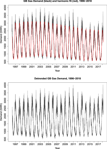
Figure 1. Upper: daily GB gas demand timeseries (black) and harmonic fit (red), April 1996–March 2018. Lower: daily GB gas demand timeseries where low-frequency variability has been removed.
Download figure:
Standard image High-resolution imageThe variation in winter mean demand is shown in figure 2 (dotted black line) and highlights a general reduction over the 22 year period. The demand variability is only weakly anti-correlated with winter mean temperature variability (r = −0.39), much lower than might be anticipated given the known drivers of gas demand. Thornton et al [2] demonstrated that low-frequency variability in both electricity and gas demand over a similar period was not driven by temperature, but was rather thought to relate to socio-economic changes over the period. Possible reasons for the reduction in gas demand over the period include more efficient gas boilers, better home insulation with more double glazing, increasing gas prices and a continued shift away from heavy industry [20].
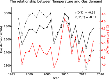
Figure 2. The winter mean of GB gas demand ('D', black dotted), demand timeseries where low-frequency variability has been removed ('Dd', solid black) and UK mean temperature ('T', red). Pearson correlation coefficients (r) are also given highlighting the much closer relationship between demand and temperature once low-frequency demand variability has been removed. The winter year is labelled according to the January and February of the winter.
Download figure:
Standard image High-resolution imageTo accurately assess the weather-driven component of gas demand and its predictability, much of the demand variability that is not driven by the weather needs firstly to be removed. Thornton et al [2] developed a methodology to remove demand variability on timescales greater than 5 years (referred to as low-frequency variability), whilst retaining demand variability on a daily, seasonal and inter-annual timescale. This approach is used here and the first step involves identifying the slowly evolving background demand. This is achieved by fitting a smoothly evolving second order Fourier expansion to the daily demand data and is shown in red in figure 1. A gradual reduction in both the annual mean gas demand and magnitude of the annual gas demand cycle is seen over the data period. This background demand is then removed from the daily demand timeseries and replaced with a climatological-mean annual demand cycle. The resultant demand timeseries, where low-frequency variability has been removed, is used in the subsequent analysis and is shown in black in the lower panel of figure 1. The highest daily demand over the data period can be seen to shift from the winter of 2003–2018 (compare upper and lower panels). Full details of the methodology to remove low-frequency demand variability are given in Thornton et al [2].
Following the removal of low-frequency demand variability, the strength of the correlation between winter mean temperature and demand increases from −0.39 to −0.87, better reflecting the known relationship [2] (see figure 2). The low-frequency variability in observed winter temperature over the 22 year period is small. Consequently, when the 5 year running mean temperature trend is removed, its correlation with demand barely changes (r = −0.85).
The predictability of two characteristics of the winter gas demand are investigated, the winter mean gas demand and the number of high demand days per winter.
2.2. Seasonal forecast data
The Met Office's global environment model (HadGEM3-GC2 [21]) consists of global models of the atmosphere, the land surface [22], the ocean [23] and sea-ice [24]. Both the operational seasonal forecast system, GloSea5 [25], and the decadal prediction system, DePreSys3 [9], are built around this same model. The atmosphere component has a resolution of 0.83° longitude and 0.55° latitude (about 60 km at mid-latitudes), with 85 vertical levels and an upper boundary at 85 km. The ocean model's resolution is 0.25° in both latitude and longitude, with 75 vertical levels.
In GloSea5 a set of retrospective forecasts, called a 'hindcast' set, is available for winters 1993–2016. Ten ensemble hindcast members are available from each calendar week. The three nearest weeks of hindcasts centred around the desired start time are collected together. For example, for a winter forecast of Dec–Jan–Feb with a one month lead time, we use the hindcast start dates of 25 October, 1 November and 9 November, giving a total of 30 ensemble members per winter. The DePreSys3 hindcast set is available for winters 1981–2018 and includes 40 ensemble members initialised on the 1 November. In both systems, ensemble member differences are created using a stochastic physics scheme [25].
Although small differences in initialisation exist between the GloSea5 and DePreSys3 hindcast sets, the two ensembles are considered to be directly comparable [5, 9], giving a combined ensemble set of 70 members for winters 1997–2016. This large size is beneficial as the prediction skill of a system typically improves with ensemble size, because the noise between ensemble members is reduced, leaving a clearer ensemble mean forecast signal [5, 26–28].
2.3. Climate predictors
Various climate indices are considered as possible predictors of winter gas demand based on atmospheric temperature or the large-scale pressure field. These climate indices are calculated for both observations and forecasts. As a proxy for observations, the gridded 6 hourly instantaneous data sets of the 'Interim' version of the ECMWF Reanalysis (ERAI [29]) are used. The data has a resolution of 0.75° longitude by 0.75° latitude and is available over the gas demand data period. Three variables are used, 2 m temperature, mean sea level pressure (MSLP) and the geopotential height of the 500 hPa pressure level (Z500). The 6 hourly data is firstly averaged to a daily mean value and then the following indices are calculated:
- Winter mean UK temperature: temperature is averaged over the region of 10°W–5°E and from 50°–60°N to give a UK mean temperature.
- Winter mean NAO: the MSLP is averaged over the regions of Iceland (63°–70°N, 25°–16°W) and the Azores (36°–40°N, 28°–20°W) [9]. For each region the winter pressure anomaly from the long term climatology is established and then the difference in these anomalies (Azores—Iceland) is determined. The same diagnostic of the geopotential height field on the 500 hPa pressure level is used to give a mid-troposphere NAO index (NAOZ500).
- Winter mean UK North–South pressure difference (ΔP): Thornton et al [3] found that the winter variation in GB daily electricity demand was strongly influenced by the regional pressure field to the north and south of the UK. An index was defined as the difference in pressure between a northern box (27°W–21°E, 57°–70°N) and a southern box (same longitudes, 38°–51°N), for regions see figure 4 in Thornton et al [3]. This is effectively a measure of the average westerly winds over the UK. This more UK centred pressure difference index is used here and a mid-tropospheric version is again calculated using the difference in the geopotential height field of the 500 hPa pressure level (ΔZ).
- Number of high demand weather type days per winter (NWT): Thornton et al [3] found that four large-scale high pressure weather patterns drive low temperatures and high electricity demand in the UK (see their figure 5). The weather types were identified by applying K-means clustering to the daily MSLP fields of the wider region. Here we explore whether predictions of the number of such days per winter is a good predictor of winter gas demand. A day is defined as a high demand weather type day if it is sufficiently similar to one of the previously identified cluster centroids. Days are included if, the sum of the absolute pressure difference across the region is smaller, and the pattern correlation is higher, than the most dissimilar day within that cluster to the cluster centroid.
The same climate indices are also calculated using the forecast data. An index is calculated for each ensemble member individually and then these are averaged to give an ensemble mean index. Due to the significant signal to noise issue when predicting the climate in the mid-latitudes [5, 26, 28], the ensemble mean climate index is used as the climate predictor, rather than the individual ensemble member values. From here onwards, 'climate index' refers to the combined ensemble mean of the climate index.
2.4. Methods for assessing forecast skill
For a climate index to be a skilful predictor of gas demand, it must have both a strong observed relationship with gas demand and be well predicted by the climate forecast system itself. Both are assessed using correlation coefficients: the Pearson correlation (rP) when the variables are continuous (e.g. winter mean gas demand, temperature) and the Spearman rank correlation (rS) if either of the variables is discrete (e.g. the number of high demand days per winter).
Skill in predicting gas demand is established by assessing the relationship strength between the forecast climate index and the observed gas demand variable, following the approach of Bett et al [16]. The ability of the climate index to predict above median, above upper tercile or the correct tercile of winter demand is assessed using the Heidke skill score (HSS).
To assess probabilistic forecast skill, a linear regression model is made between observed winter mean demand and the forecast climate index. The skill of probabilistic forecasts for the demand categories above can then be assessed, using the Brier and rank probability skill scores (BSS and RPSS respectively), employing leave-one-out cross validation. A preliminary assessment of the reliability of the probabilistic forecasts is also given. For a comprehensive description of the different statistical measures see Wilks [30].
3. Results
3.1. Using temperature as a predictor of winter mean gas demand
Figure 3 summarises the prediction skill of winter mean gas demand using temperature as the predictor. As discussed previously, observed winter mean temperature is strongly anti-correlated with GB winter mean gas demand (rP = −0.87, see figure 3(a), this is a repeat of figure 2, and is included to allow comparison with the predictions). The skill in forecasting winter mean temperature across North-western Europe and the Atlantic is shown in figure 4. Temperatures are skilfully forecast over many areas of the North Atlantic and over Scandinavia. In contrast there is little skill over continental Europe. Much of the skill over the ocean is however related to the low-frequency warming trend, such that when the 5 year running-mean winter-mean temperature trend is removed the prediction skill is negligible over most of the North Atlantic (not shown). There is significant skill in predicting the average temperature over the UK region, but the correlation magnitude is still relatively small (rP = 0.38, see table 1 and figure 3(b)). A similar skill level is found when a 5 year running-mean temperature trend is removed.
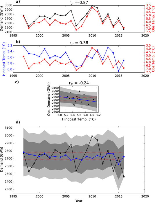
Figure 3. Using temperature to predict winter mean gas demand. (a) Timeseries of the winter mean GB gas demand and winter mean temperature. (b) Timeseries of winter mean temperature and winter mean hindcast temperature. (c) Regression relationship between hindcast temperature and observed demand (blue), the prediction interval (central 95%-light grey, central 75%-dark grey), and the observed terciles of gas demand are shown (red dashed lines). (d) Timeseries of winter mean gas demand (black) and central regression prediction (blue) and prediction interval (grey). The Pearson correlation coefficients (rP) are given for (a)–(c). Note, the temperature axes are inverted in (a) and (b) to allow easier comparison with gas demand.
Download figure:
Standard image High-resolution image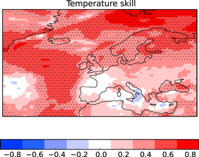
Figure 4. Map of the winter mean temperature forecast skill: the Pearson correlation coefficient between hindcast and observed temperature. Statistically significant skill at the 5% level is shown by stippling using a 1-sided Fisher Z test.
Download figure:
Standard image High-resolution imageTable 1. Column 1: Pearson correlation coefficient (rP) between winter mean gas demand (Dobs) and observed winter mean climate index (Cobs). Column 2: the hindcast skill in predicting the climate index (correlation of observed and hindcast climate index). Column 3: the hindcast skill in predicting winter mean gas demand (magnitude of correlation between Dobs and Chc). All data considers winters 1997–2016. Bold values indicate the correlation is significant at the 5% level using a 1-sided Fisher Z test.
| Climate Index | Obs relationship | Climate index | Gas demand |
|---|---|---|---|
| (C) | rP (Dobs, Cobs) | skill, rP (Cobs, Chc) | skill,  (Dobs, Chc) (Dobs, Chc) |
| Temperature | −0.87 | 0.38 | 0.24 |
| NAO | −0.62 | 0.63 | 0.40 |
| NAOZ500 | −0.66 | 0.63 | 0.55 |
| ΔP | 0.70 | 0.60 | 0.49 |
| ΔZ | 0.71 | 0.58 | 0.57 |
| NWT | 0.66 | 0.56 | 0.57 |
A forecast of UK average winter mean temperature is not found to be a good predictor of winter mean gas demand. Although the Pearson correlation coefficient between the hindcast temperature and observed demand has the correct sign (negative), its low magnitude ( ) means it is not statistically significant at the 5% level. A large spread in the relationship can be seen in figure 3(c), leading to little variation in the probabilistic prediction of winter mean demand from year to year (figure 3(d)). Although the deterministic HSSs are positive for above median and above upper tercile demand, the equivalent probabilistic skill scores are worse or similar to those of a climatological forecast (e.g. RPSSter = 0.03, see table 2). In summary, although temperature variability drives a significant proportion of demand variability, forecast temperature is not a good predictor of winter mean gas demand due to the limited skill in predicting UK temperatures.
Table 2. A summary of verification skill scores for predicting winter mean gas demand when using the different climate predictors. The Heidke skill score (HSS), the Brier skill score (BSS) and the ranked probability skill score (RPSS), for above median demand (med), above upper tercile demand (upper) and considering all terciles (ter). Scores greater than zero indicate the forecast is better than random chance (in the case of the HSS) and better than a climatological forecast for the BSS and RPSS, following Wilks [30]. Bold (Italics) signifies the score is significant at the 5% (10%) level. Significance is assessed using a 1000 member bootstrap, where the skill score is calculated between the observed demand timeseries and a randomly sampled (without replacement) hindcast timeseries. A value is significant if it is greater or equal to the 95th (90th) percentile of the bootstrap distribution.
| Climate index | HSSmed | BSSmed | HSSupper | BSSupper | HSSter | RPSSter |
|---|---|---|---|---|---|---|
| Temperature | 0.40 | 0.09 | 0.12 | −0.13 | 0.25 | 0.03 |
| NAO | 0.40 | 0.18 | 0.56 | 0.12 | 0.32 | 0.18 |
| NAOZ500 | 0.40 | 0.26 | 0.78 | 0.41 | 0.40 | 0.33 |
| ΔP | 0.60 | 0.19 | 0.56 | 0.18 | 0.32 | 0.26 |
| ΔZ | 0.40 | 0.28 | 0.56 | 0.30 | 0.47 | 0.32 |
| NWT | 0.60 | 0.33 | 0.78 | 0.30 | 0.62 | 0.34 |
3.2. Using the atmospheric circulation as a predictor of winter mean gas demand
All circulation-based indices (NAO, NAOZ500, ΔP, ΔZ and NWT) have a strong observed relationship with winter mean gas demand (rP of ∼0.6–0.7, see table 1, column 1). However none of the circulation indices have as strong a relationship with demand as winter mean UK temperature.
The skill in predicting the winter MSLP across North-western Europe and the wider North Atlantic is shown in the left panel of figure 5. Skill is found at both high (60°–70°N) and low (30°–40°N) latitudes. In contrast, over the mid-latitudes (40°–60°N) including over the UK there is not significant prediction skill. A similar picture is seen for the Z500 field (figure 5, right). Nevertheless, skilful predictions of the winter mean circulation indices are possible (rP ∼ 0.6, see table 1, column 2), as the indices measure the difference in pressure between the skilfully predicted low and high latitude regions. This skill is important because it is the gradient in pressure which drives surface weather conditions. The total number of high demand weather type days per winter is also skilfully predicted at the 5% level (rP = 0.56). This weather type skill effectively demonstrates skill in predicting the frequency of days where high pressure influences the UK in winter and is consistent with previous studies [8].

Figure 5. Map of the winter mean forecast skill for MSLP (left) and 500 hPa geopotential height (right): the Pearson correlation coefficient between the hindcast and observed fields from 1994–2016. Statistically significant skill at the 5% level is shown by stippling using a 1-sided Fisher Z test.
Download figure:
Standard image High-resolution imageWinter mean gas demand is skilfully predicted when using any of the circulation indices as the predictor, with correlations between hindcast index and observed demand ranging from approximately 0.4–0.6 (see table 1, column 3). Predictions of winter mean demand greater than the median or upper tercile are skilful, showing improvements over using a random or climatological forecast (scores often exceeding 0.25, see table 2). For below lower tercile demand all predictors give positive HSSs (∼0.3–0.6), however only NAOZ500, ΔP and ΔZ give skilful probabilistic forecasts (BSSs of 0.05–0.12). This suggests a possible asymmetry, with better forecast skill for higher demand winters than lower demand winters, which could be beneficial given their larger impact.
Figure 6 demonstrates the skill in predicting winter mean gas demand using ΔZ as the climate predictor. The strong observed relationship between ΔZ and demand is shown in figure 6(a), and the prediction skill of ΔZ is shown in figure 6(b). A significant linear relationship exists between observed demand and hindcast ΔZ (r = 0.57, see figure 6(c)), leading to a variation in the forecast of gas demand from year to year (figure 6(d)). The probability of above median demand, above upper tercile demand, and the correct tercile category is skilfully forecast and better than using a climatological forecast (BSSmed = 0.28, BSSupper = 0.30, RPSSter = 0.32). Use of the linear regression model between hindcast climate index and observed demand, means forecasts are automatically bias adjusted and probabilities are reliable, for example see figure 7. Due to the small number of winters available, the reliability is only assessed across 4 probability bins. An operational forecast could therefore present the risk of an event using 4 categories, e.g. the probability (P) of above tercile demand is 'low' (P < 0.25), 'below median' (0.25 ≤ P < 0.5), 'above median' (0.50 ≤ P < 0.75) or 'high' (P ≥ 0.75), rather than giving actual probabilities.

Figure 6. Using the winter mean Z500 North–South height difference (ΔZ) to predict winter mean gas demand. (a) Timeseries of the winter mean GB gas demand and ΔZ. (b) Timeseries of observed and hindcast ΔZ. (c) Regression relationship between hindcast ΔZ and observed demand (blue) and the prediction interval (grey). (d) Timeseries of winter mean gas demand (black) and central regression prediction (blue) and prediction interval (grey). See figure 3 for details.
Download figure:
Standard image High-resolution image
Figure 7. Reliability diagrams for probabilistic forecasts of winter mean gas demand using ΔZ as the climate predictor, for above median (left) and above upper tercile (right) demand. A perfectly reliable forecast would lie along the 1:1 line (black). The sample climatological probability is also given (red dotted). The lower bar charts show the distribution of forecast probabilities made during the hindcast period, ideally these would be flat, with each probability bin well sampled.
Download figure:
Standard image High-resolution imageTo explore how many ensemble members are needed to ensure a skilful forecast of gas demand, figure 8 shows how the prediction skill varies with ensemble size. Increasing the ensemble size from 1–30 leads to a rapid increase in prediction skill (the correlation increases from ∼0.1–0.5). Increasing the ensemble size even more leads to further improvements in the prediction skill, but at a much slower rate. Nevertheless, higher skill would likely be possible with more members.
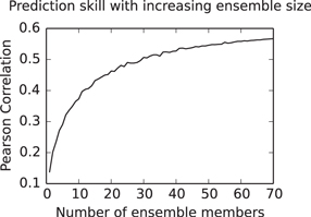
Figure 8. The impact of ensemble size on hindcast skill, when predicting winter mean gas demand using winter mean ΔZ. The skill is measured using the Pearson correlation coefficient. 1000 samples of the correlation have been generated by randomly sampling the ΔZ ensemble members each winter, to give alternative hindcast ensemble mean timeseries. The mean correlation of the bootstrap samples is shown. For a sample size of 20, statistical significance at the 5% level using a 1-sided Fisher Z test, is achieved with a correlation of at least 0.379.
Download figure:
Standard image High-resolution imageIn summary, skilful prediction of winter mean gas demand is possible using a forecast of the winter mean atmospheric circulation. The improvement over using a temperature forecast occurs because of the better prediction skill of the circulation indices. The circulation indices are calculated over a much larger area compared to the temperature index, which may explain their better skill.
3.3. Predicting the number of high gas demand days over the winter period
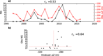
A day is classed as a high demand day if its demand is equal to or greater than the 95th percentile of daily winter demand calculated over all winters. Between 1997–2016 the observed number of high gas demand days per winter ('NG') varies between 0–15 (see black line, figure 9(a)). As these events stress the energy supply system an obvious question is whether their likelihood is predictable ahead of the winter. There is a strong correlation between winter mean gas demand and NG (rS = 0.70). Consequently, if mean demand is skilfully predicted, NG may also be predictable to some extent.
Figure 9. Using atmospheric circulation to predict the number of high gas demand days per winter (NG). (a) Observed timeseries of NG and winter mean ΔZ. (b) The relationship between hindcast ΔZ and observed NG. The median count and hindcast ΔZ are indicated with a dotted red line. The Spearman rank correlation coefficients are also given (rS).
Download figure:
Standard image High-resolution image
Although observed winter mean temperature has a reasonable relationship with NG (rS = −0.55), temperature is not a useful predictor of NG (rS = −0.11 between NG and hindcast winter mean temperature, see table 3, column 2). All circulation indices do however give skilful predictions of NG, with Spearman rank correlation magnitudes of approximately 0.4–0.6 (same table).
Table 3. Column 1: Spearman rank correlation coefficient (rS) between observed NG (NGobs) and observed winter mean climate index (Cobs). Column 2: hindcast skill in predicting NG (correlation magnitude between NGobs and Chc). All data considers winters 1997–2016. Bold values indicate the correlation is significant at the 5% level using a 1-sided Fisher Z test.
| Climate Index | Obs relationship | NG skill |
|---|---|---|
| (C) | rS (NGobs, Cobs) |
 (NGobs, Chc) (NGobs, Chc) |
| Temperature | −0.55 | 0.11 |
| NAO | −0.49 | 0.42 |
| NAOZ500 | −0.47 | 0.63 |
| ΔP | 0.54 | 0.54 |
| ΔZ | 0.53 | 0.64 |
| NWT | 0.55 | 0.57 |
A demonstration of the prediction skill of NG, using winter mean ΔZ as the predictor, is shown in figure 9. Given NG is discrete and limited to positive numbers, linear regression is not suitable for modelling its relationship with ΔZ. Due to the small sample size there is also considerable uncertainty in the form of the relationship between observed ΔZ and the NG. Consequently we do not try to model the relationship, rather we assess the prediction skill using a deterministic approach. Figure 9(b) shows the relationship between hindcast ΔZ and observed NG. As the predicted atmospheric flow over the UK becomes less westerly (i.e. ΔZ becomes less negative), NG increases. The contingency table for above median counts show that the hit rate is far higher than the false alarm rate (see table 4), leading to a HSS of 0.6 (statistically significant at the 5% level using a 1000 member bootstrap as per table 2). For above upper tercile counts, the HSS is positive (HSS = 0.34) but it is not statistically significant at either the 5% or 10% levels. Very similar results are found for the other atmospheric circulation predictors, whilst a temperature based prediction is no better than when using a random forecast (HSS ≤ 0).
Table 4. Contingency table for above median count of the number of high demand days per winter, using ΔZ as the predictor.
| Above median | Observed | ||
|---|---|---|---|
| Count | Yes | No | |
| Predicted | Yes | 8 | 2 |
| Hits | False alarms | ||
| No | 2 | 8 | |
| Misses | Correct rejections | ||
| Hit rate: | 80% | ||
| False alarm rate: | 20% | ||
In summary, given a forecast of the atmospheric circulation, we can give a skilful forecast of above median counts of the number of high gas demand days per winter. A longer timeseries is needed to assess the predictability of winters with a higher number of high demand days.
4. Conclusions
The predictability of the weather-driven component of Britain's winter gas demand is assessed from early November using a range of climate predictors. Two components of gas demand are considered: winter mean gas demand and the number of high demand days over the winter period. The forecast skill is analysed from 1997–2016 using a large ensemble of retrospective climate forecasts from the Met Office's seasonal and decadal prediction systems. The climate predictors analysed are winter means of temperature, the NAO and a UK centred North–South pressure difference (at the surface and in the mid-troposphere). An additional predictor, based on the frequency of high demand weather types over the winter period, is also analysed. Forecast skill is assessed using a range of deterministic and probabilistic skill measures with a focus on the risk of higher demand winters. The main conclusions are:
- All circulation-based indices give skilful forecasts of winter mean gas demand. This is because such indices are both strongly correlated with gas demand and are skilfully predicted ahead of the winter period.
- A method for giving operational gas demand forecasts is demonstrated, based on a regression relationship between the climate predictor and observed gas demand. Skilful and reliable probabilistic forecasts of the risk of above median, above upper tercile and the correct tercile of winter mean demand are possible.
- A large ensemble of hindcast members is needed to give a skilful prediction of winter mean gas demand, reflecting the known signal to noise problem of seasonal forecasting in the Atlantic sector.
- Although winter mean temperature is the climate index most highly correlated with winter mean gas demand, due to the lower seasonal prediction skill of temperature, it does not give skilful predictions of winter mean demand.
- A skilful forecast of above median counts of the number of high gas demand days per winter is possible using a forecast of the winter mean atmospheric circulation.
The skilful prediction of winter gas demand demonstrated here, offers the potential for improved planning and resilience of Britain's energy system. For example, a more accurate forecast of winter demand could reduce the risk of gas supply shortages and related energy price spikes. It would be of interest to assess the skill of winter demand forecasts with a longer lead time, for example from early September or October, and when averaged over a shorter period, such as individual months, as both would clearly be useful. The use of atmospheric circulation to predict energy demand could also give skilful forecasts in other regions, provided demand is driven by the weather and skilful circulation forecasts are available. Seasonal weather forecasts offer the first outlook for the coming winter, but should be used in conjunction with other nearer term forecasts, such as monthly outlooks through to day ahead forecasts, to maximise the preparedness of the energy industry for extreme demand events.
Acknowledgments
We thank Simon Geen from National Grid for providing the gas demand data set and Paul Newell and Simon Brown at the Met Office for useful discussions. This research was supported by the Met Office Hadley Centre Climate Programme funded by BEIS and Defra, the 'European Climatic Energy Mixes' project (ECEM), a Copernicus Climate Change Service (2015/C3S_441_Lot2_UEA) and the European Union's Horizon 2020 research and innovation programme under grant agreement No 776868 (SECLI-FIRM project).