

Abstract
Systematic errors in forecast near-surface air temperature (SAT) still constitute a considerable problem for numerical weather prediction (NWP) at high latitudes. Numerous studies in the past have attempted to reduce this problem through recalibration of physical parameterization schemes and better approximation of the surface energy budget. The errors, however, remain despite notable improvements in the overall weather forecast performance. This study looks at the problem from a different perspective. It analyzes asymmetries in the SAT forecast errors. The study reveals a statistical pattern of warm SAT biases under cold weather conditions and cold SAT biases under warm weather conditions. The largest errors were found in shallow atmospheric boundary layers (ABLs). The study attributes the problem to the modeled excessive ABL thickness in northern Eurasia (the NEFI region). The ABL thickness is considered as a scaling factor controlling the efficacy of the applied surface heating. Too thick an ABL damps the magnitude and agility of the SAT response. The study utilized the operational model SL-AV of the Russian Hydrometeorological Centre. Two turbulence schemes were evaluated in the northern European and western Siberian regions of Russia against observations from 73 meteorological stations. The pTKE (old) scheme is based on the local balance of the turbulence characteristics. The TOUCANS (new) scheme incorporated the total turbulence energy equations in an energy-flux balance approach. Neither scheme uses the ABL thickness as a prognostic parameter. The study reveals that the SAT errors are consistent with the damped response of temperature and reduced agility of temperature fluctuations in too thick ABLs. The TOUCANS scheme did not improve those features, probably because it links the turbulent fluxes and the ABL thickness. The SAT errors in shallow ABLs persist in the new scheme. This study emphasizes the need for a closer look at the ABL thickness in the NWP models.
Export citation and abstract BibTeX RIS

Original content from this work may be used under the terms of the Creative Commons Attribution 3.0 licence. Any further distribution of this work must maintain attribution to the author(s) and the title of the work, journal citation and DOI.
1. Introduction
Accurate forecasting of air temperature at the standard 2 m height above the ground (the near-surface air temperature or SAT) is an important task for operational numerical weather prediction (NWP). The SAT forecast by NWP models is still imperfect. The errors in SAT remain stubborn despite numerous attempts to approach the problem from different perspectives over a few decades (Sandu et al 2013; hereafter referred to as S13). These errors have resisted model improvement efforts, especially in cold climate regions over the northern continents and in the Arctic (Vogelezang and Holtslag 1996, Atlaskin and Vihma 2012, Holtslag et al 2013, Kleczek et al 2014, Groisman et al 2016, Batrak and Müller 2018). The challenge for SAT modeling in cold regions was highlighted, among other calls for coherent studies and new observations, during the Year of Polar Prediction (YOPP) as stated by, for example, Jung et al (2016). A more robust SAT forecast is also needed for sustainable development of the northern Eurasian territories and improving the resilience of the northern settlements, as stated in the research strategy of the North Eurasia Future Initiative (NEFI) (http://www.neespi.org/NEFI-WhitePaper.pdf; Soja and Groisman 2018), the Pan-Eurasian Experiment (PEEX) (https://www.atm.helsinki.fi/peex/index.php; Lappalainen et al 2016) and in the Arctic Megatrends report (Karlsdóttir 2011).
The stubborn resistance of SAT errors has been traced to parameter constraints of turbulence schemes and inaccuracies of the surface energy budget in numerical models (Tjernstroem et al 2005, Vihma et al 2014, Sterk et al 2016). More detailed analysis of convective and stably stratified atmospheric boundary layers (CBL and SBL, respectively) revealed that a shallow SBL induces significantly larger SAT biases in response to a given anomaly of the surface energy budget (Cuxart et al 2006, Svensson et al 2011, Esau et al 2012, Kleczek et al 2014). Consequently, the largest SAT errors are found in geographical regions with cold climate and during prolonged periods (night- and winter-time) with a negative surface energy balance (Davy and Esau 2014). Repeated attempts to correct and improve the schemes have had only limited success (Brown et al 2008, S13, Pithan et al 2015). We argue in this study that the existing focus on local turbulence properties, for example on stability correction functions (Kleczek et al 2014), is perhaps too restrictive to meet the challenge.
This study is based on a series of forecasts with the operational semi-Lagrangian—absolute vorticity equation (SL-AV) NWP model of the Russian Hydrometeorological Centre (Tolstykh et al 2015). We question whether the scaling factor, which is given by the thickness of the atmospheric boundary layer (ABL),  is significantly related to the systematic SAT errors found in the numerical weather forecast over northeastern Europe and western Siberia. This region has been chosen for the study as it is included in the NEFI focus area, and it is covered with sufficient number of meteorological stations to run a statistically representative analysis. To answer this question, we describe a set of expected effects on the SAT differences, which could be induced by misrepresentation of
  in the models. Then, we search for those effects in the operational weather forecasts for January 2015 over these regions.
The paper is organized as follows. The next section introduces the concept and methods of this study. Section 3 describes the NWP model, emphasizes the relevant differences in the pTKE and TOUCANS turbulence schemes and presents the numerical experiments. Section 4 reports and discusses the results. The final section highlights the conclusions of the study.
2. A new perspective on turbulence scheme analysis
2.1. ABL thickness as a scaling factor
This study introduces and explores a new perspective on SAT error analysis in the context of ABL modeling. This perspective emerges from an underappreciated factor, which scales forcing efficacy by the ABL thickness,  Let us look at the following simple energy-balance equation (e.g. Park et al 2005, Zilitinkevich and Esau 2009, Rypdal 2012, Davy et al 2017):

Usually, for example in Rypdal (2012),  is understood to be the mean temperature of a bulk well-mixed layer of thickness
  and constant heat capacity
  However, it is known that in a well-mixed layer, the temperatures at any layer, and also the SAT, are functionally dependent. This is a trivial fact for a CBL where
  and
and  is an adiabatic temperature gradient. This is less trivial in a SBL where more sophisticated relationships apply (Zilitinkevich and Esau 2005). The coefficient
  should account for the weaker mixing in a SBL where
  Following the accepted methodology of turbulence studies, we understand equation (1) in a statistical sense as valid only on average. Here,
  is the SAT difference (error) in the model, i.e. the deviation of the model SAT value
  from the corresponding collocated observed value
  This deviation is caused by a proper energy imbalance
  in the model. In terms of equation (1),
  is the surface turbulent sensible heat flux anomaly. In the NWP model, this anomaly could be caused by errors in other components of the heat budget, which modify the sensible heat flux through the surface energy-balance equation.
This SAT response,  is scaled by the effective heat capacity of the system, which could be expressed through
  In the ABL, the energy imbalance
  is changing the atmosphere through vertical turbulent exchange. The fact that the turbulent exchange is faster than the advective or radiative changes has been also used in the construction of turbulence schemes in the NWP models. We will consider two such schemes in this study. In an operational NWP model, the SAT differences can be also of a dynamic origin. We acknowledge this difficulty, but do not consider it in this research letter.
In the studied regions of northern Russia, most, if not all, land is covered with snow in January. The snow acts as insulator inhibiting heat exchange between the atmosphere and the soil. The data used in this study show that the observed daily maximum temperature slightly exceeds 0 °C at some stations on some days in the north European part of Russia; however, the daily minimum temperature is always below 0 °C except for 1–3 of January for three stations. In Siberia, there are only few occasional positive daily maximum temperatures, all daily minimum temperatures being negative. This means that soil and, in particular, soil wetness effects do not play any role in the SAT differences.
The ABL thickness,  is a scaling factor moderating the temperature response,
  on the proper energy imbalance,
  Cuxart et al (2006) and Beare et al (2006) demonstrated that
  could be as much as an order of magnitude larger in the turbulence schemes than in the corresponding observations or in turbulence-resolving large-eddy simulations. A small scaling factor makes SAT sensitive even to small energy imbalances. Contrary, a large
  damps the SAT sensitivity even to large imbalances. The scaling factor does not determine the sign of the temperature response. Davy and Esau (2014) found that the majority of climate models maintain ABLs that are too thick, particularly over continents and at high latitudes, where the observed ABLs are naturally shallow due to the mostly negative surface heat balance (Serreze et al 2007) and stronger stability of the lower atmosphere (Medeiros et al 2011, Zhang et al 2011).
2.2. Constraints on the magnitude of the SAT response imposed by the scaling factor
It needs to be clarified that the scaling factor  in equation (1) should not be considered as yet another underrepresented component of the surface energy budget. This is a factor which scales
  to some degree independently of its nature. We acknowledge that some errors in the heat budget would be correlated with
  For instance, radiative effects of the convective cloud cover are likely to be correlated with large
  in the thick convective boundary layer. Detailed investigations of such correlations require a separate study, being outside of scopes of this letter.
Our previous studies of the climate models and ERA interim reanalysis (Esau et al 2012, Davy and Esau 2014, Davy et al 2017) convinced us that  scaling as such could be studied statistically with no regard to the intrinsic physical structure of the forcing. The ABL thickness varies by an order of magnitude from
  in a SBL to
  in a CBL. Therefore,
  that is well correlated with the SBL events will be significantly more amplified. Thus, if the SAT difference is indeed sensitive to
  some kind of a reciprocal relationship
  should surface in the NWP data. To reveal such dependences, we will transform the data from the traditional analysis of
  to an analysis of
It is possible to demonstrate that the differences in  introduce a specific statistical signature. Unfortunately, the ABL thickness is not available from routine ground-based meteorological observations. Its determination from radiosounding data provides rather uncertain values, which are sensitive to the choice of method and the stability of the lower atmosphere (e.g. Seibert et al 2000, Seidel et al 2012, Wang and Wang 2016). Therefore, the observed and modeled
  could be compared only in special idealized studies, for example in the GEWEX Atmospheric Boundary Layer Study (GABLS) (Cuxart et al 2006, Svensson et al 2011), where the effects of intermittency and statistics of the cooling/warming events are not considered. The operational weather forecast generates such statistics providing an opportunity to study the SAT errors in ABLs of significantly different thickness.
2.3. Low-pass filtering effects of the scaling factor
The scaling factor not only modifies the amplitude of the response, but also imposes low-pass filtering on it (Rypdal 2012). Equation (1) has the following solution in response to a delta-pulse forcing 

where  is a combined diabatic sensitivity parameter (Park et al 2005). It follows that
  in the shallow SBL will not only be amplified but will also show a more agile response and will respond to more high-frequency external fluctuations than a thick CBL. Considering realistic chaotic forcing, the low-pass filtering in equation (2) creates a biased memory effect on the SAT. Slower fluctuations are better captured by a thick ABL. Too large an
  in the model should induce larger SAT differences during periods with more rapid heating fluctuations. Thus, stable anti-cyclonic conditions with a pronounced diurnal cycle of
  should result in a larger
  than the conditions with dominating synoptic variability. The low-pass filtering induces insufficient diurnal range in the models. The damped modeled temperature range was found in comparisons with satellite temperature products (Liu et al 2006) and with in situ data (Yang et al 2006). Although these kinds of errors are difficult to disentangle, a look at the probability density function (PDF) may provide a useful clue to the scale of the effects (Ashkenazy et al 2008). This effect will be observed even in the situation of a perfectly modeled surface energy budget.
The SAT itself could be used for rough estimation of  (for momentum) as Esau et al (2012) have demonstrated. Indeed, a shallow SBL is created by surface cooling or warm air advection. Those conditions lead to a lower temperature of the surface than of the air above it. In contrast, a deep CBL is created by surface warming or cool air advection. Statistically, the dependence
  could be transformed to
  The latter is easier to study in comparison with the observational data. Previous studies, for example the evaluation by Atlaskin and Vihma (2012) of four NWP models, demonstrated that
  increases with decreasing temperature and strengthening of the low-level temperature inversions. They also noted the low-pass filtering of the forcing fluctuations as the models responded too slowly in situations of rapid drops in temperature. The magnitudes of SAT tendencies in the models were only 17%–20% of the observed magnitudes. A similar slow response was noted in Beesley et al (2000). Fay and Neunhauserer (2006) demonstrated that the slow response and warm bias in their limited area model forecast did not disappear even in very high-resolution (1 km) runs.
3. The NWP model and numerical experiments
3.1. The SL-AV model configuration
The SL-AV global atmospheric general circulation model (Tolstykh 2003, Tolstykh et al 2015) is used for operational medium-range numerical weather prediction, and is applied as a component of the probabilistic long-range forecast system at the Hydrometeorological Centre of the Russian Federation (HMCR). The model is based on a semi-Lagrangian semi-implicit dynamical core, which has been developed and described by Tolstykh et al (2017). The model uses a stretched latitude–longitude grid with a locally refined resolution over Russian territory (Tolstykh et al 2017). The original SL-AV dynamical core uses the vertical component of the absolute vorticity and divergence as prognostic variables. It employs fourth-order finite differences at the unstaggered grid to approximate non-advective equations terms. In this study, we use the operational version of the SL-AV model for medium-range weather forecasts with the resolution in latitude varying from 0.155° to 0.178° in the Northern Hemisphere to 0.24° in the Southern Hemisphere. The resolution in longitude is 0.225°; the model has 51 vertical levels with the highest model level placed at 5 hPa, with 10 levels being located in the lowermost kilometer of the model atmosphere.
Physical processes in the SL-AV at unresolved scales are parameterized mostly using the algorithms developed by the mesoscale weather prediction consortium ALADIN/LACE (Termonia et al 2018). Shortwave and longwave radiation is calculated using CLIRAD SW (Chou and Suarez 1999, Tarasova and Fomin 2007) and RRTMG LW (Mlawer et al 1997) algorithms, respectively. Some parameterizations of important physical processes, for example a multilevel soil model by Volodin and Lykossov (1998), were developed in addition to the standard version.
3.2. Turbulence parameterization schemes in the model
The SL-AV forecast was run with two different ABL schemes, which we will refer here to as the old scheme and the new scheme. Both schemes provide a diagnostic estimate of the ABL height. The old scheme is also known as the pTKE scheme. We will briefly present the central elements of these schemes following Geleyn et al (1994), Redelsperger et al (2001), Geleyn et al (2006) and Bašták Ďurán et al (2014), hereafter referred to as BD14. A reader seeking for an exhaustive description should refer to those publications.
The old scheme is based on a version of the scheme of Louis (1979) in which advection and self-diffusion of the turbulent kinetic energy (TKE) is computed by the level 2.0 Louis-type scheme taken to be the stationary solution of the system with unresolved fluxes. The latter conditions mean that the TKE is obtained from the turbulent exchange coefficients following the procedure in Redelsperger et al (2001). The ABL thickness,  is a diagnostic parameter, and is calculated following the approach of Troen and Mahrt (1986) modified by in an iteration scheme by Ayotte et al (1996). The ABL thickness is calculated as

where  is the critical the bulk Richardson number formulated using the difference between the surface temperature and the temperature at the top of the mixed layer,
  are the components of the horizontal velocity,
  are the potential temperatures at the top of the ABL and at the surface and
  is the acceleration due to gravity. Equation (3) is tried for different model levels starting from the lowermost one until the bulk Richardson number becomes larger than the prescribed
  It is used to calculate the mixing length scale,
  at different elevations above the surface. The corresponding equation is shown below to demonstrate that
  and therefore the turbulent fluxes, decay smoothly with the height,
  but are not confined within the layer of thickness
  :
:
Here,  is the von Karman constant and
  are the tuning constants. Thus, a direct modification of the ABL thickness in this scheme is hardly possible. Moreover, the effects of such modifications will not be straightforward to evaluate as the turbulent fluxes cannot be adjusted independently of
An important structural feature of turbulent mixing in a SBL as described in Zilitinkevich et al (2013), is the fact that the velocity and temperature fluctuations are differently transferred by the turbulent motions in the stably stratified fluid flow. Stability damps the vertical velocity fluctuations,  but it simultaneously increases the temperature fluctuations,
  as the temperature gradients increase. As a result, the temperature flux,
  remains significant even in very stably stratified flows. There are two effective consequences of this feature: the ABL thickness is not directly proportional to the stability of the layer—it are linked through a non-constant turbulent Prandtl number, Pr; and vertical heat mixing remains significant in a shallow SBL but rapidly vanishes above it. This better understanding lead to a new energy-flux balance (EFB) family of parameterization schemes.
A Third Order moments Unified Condensation Accounting and N-dependent Solver for turbulence and diffusion (TOUCANS) scheme was proposed in BD14. A variant known as the eeEFB scheme is referred to as a new scheme in this study. The new scheme is based on a compact model for the stability dependence of the turbulent kinetic energy without a critical Richardson number. It is based on an analytical framework combining and simplifying the revisited Mellor–Yamada formulation (Canuto et al 2008) and the EFB approach (Zilitinkevich and Esau 2007, Zilitinkevich et al 2013). Significant changes were introduced in the formulations of the stability correction functions. An essential feature of the new scheme is the use of the total turbulent energy (TTE) as a prognostic variable. The TTE is a sum of the TKE and the turbulent potential energy, which is given by the squared temperature fluctuations,  The TOUCANS formulation is valid for all stability conditions, and accounts for turbulence anisotropy in both momentum- and heat-related terms. The TOUCANS parameterization also accounts for the third-order moments for unstable stratification. The mixing length is calculated in the same way as in the old scheme (equation 3).
3.3. Setup and conditions of the numerical experiments
The SL-AV model was set to compute 27 h global forecasts starting from the HMCR operational analyses for each day of January 2015 at 12:00 UTC. The forecast data for lead times from 6 to 27 h are stored with a time step of 3 h. The forecast data for the first 6 h are dropped to exclude possible spinup effects. Longer lead times are excluded from our consideration as 'slow' diabatic processes (e.g. radiation) play a more important role for these times. The SL-AV model was run with both old and new boundary layer schemes providing two forecast series. All other model settings were identical in both series. The forecast SAT and  were interpolated into locations of selected meteorological stations using the bilinear interpolation method.
The chosen region of northern Russia (figure 1) is a rather homogeneous and flat region. Only a small fraction of it is occupied by the Khibiny and Urals mountains. To maintain homogeneity of our analysis, meteorological observations from elevated stations were not considered. We also exclude several arctic coastal stations as the current model grid does not represent their surface type correctly. We include only those stations that provided eight SAT observations every day between 1 and 31 January 2015 without missing and wrong values. Wrong values are defined as those that differing by more than 12 K from the observed values 3 h before and 3 h later. The whole region was broken in two distinct climatic sub-regions, namely the region of the northern European part of Russia (58°–70° N, 30°–55° E) with a temperate continental climate and more clouds and the western Siberian part (55°–75° N, 60°–85° E) with a severe continental climate and fewer clouds. A description of the prevailing meteorological situation in January 2015 in these sub-regions is presented in the supplementary material (available online at stacks.iop.org/ERL/13/125009/mmedia). In total, we considered 33 meteorological stations in the European part and 40 stations in Siberia.

Figure 1. The regions of the northern European part and western Siberian part of Russia (the NEFI region) where the SAT forecast errors in the SL-AV NWP were studied. The meteorological stations are shown with circles. The colors correspond to the mean SAT errors,  averaged over the diurnal cycle, in January 2015 in the forecasts with the old (pTKE) scheme. Figure S5 in the supplementary material presents the data obtained with the new (TOUCANS) scheme. The circle size indicates the monthly mean ABL thickness in the model. The black ring marks the selected WMO station with ID 28573.
Download figure:
Standard image High-resolution image4. Results and discussion
This study reports the analysis of two series of 31 daily forecasts for January 2015 produced by the operational SL-AV NWP model. The conventional analysis would look at different components of the surface heat budget searching for their connections with the turbulence scheme parameters and relationships, as was discussed and criticized for example in S13 and BD14. Here, the analysis is focused on tracing plausible effects due to misrepresentation of the ABL thickness,  Figure 2 demonstrates co-variability of the observed and forecast quantities at one selected meteorological station (WMO ID 28573) from the Siberian region. Such figures for all stations can be found in the supplementary material. The prepared data and visualization routines are available by request from the corresponding author.
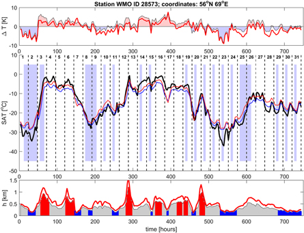
Figure 2. Observations and model predictions of the SAT, h,  and the surface heat budget from the selected Siberian station with WMO ID 28573. The SAT is shown in the central panel. The three curves are: the observed temperature (black); the SAT predicted with the old (pTKE) scheme (blue); the SAT predicted with the new (TOUCANS) scheme (red). Blue shading shows the periods of time with a negative modeled surface heat budget accumulated over 6 h in the prediction with the old scheme. The vertical dashed lines mark the end of the calendar days (from 1 to 31 January 2015). The differences,
  between the observed and predicted SAT are shown in the upper panel. Color shading shows
  for the prediction with the old scheme. The red curve shows
  for the new scheme. The ABL thickness, h, is shown on the lower panel. Color shading shows h for the old scheme and the red curve for the new scheme. Blue bars highlight episodes of a shallow SBL (
 ) and red bars episodes of a thick ABL (
 ). All data were resampled at 3 h intervals.
Download figure:
Standard image High-resolution image4.1. Analysis of the SAT errors at a selected station
The considered meteorological quantities varied widely during the period of the study. This variability provides us with representative statistics of advection- and radiation-dominated synoptic conditions. The first half of the month experienced a transient synoptic activity with large (up to 30 °C) but slow SAT variations. The surface heat budget changed relatively slowly with a characteristic time scale of several days. The second half of the month experienced more persistent anti-cyclonic conditions with cold temperatures. The changes in the surface heat budget were dominated by the diurnal cycle. The diurnal temperature range was small due to low winter-time solar elevation at these latitudes.
The temperature difference,  between the observed,
  and predicted,
  SAT also varied considerably. The variations are not chaotic but tend to fell in two bins. One bin is characterized by a shallow ABL (the blue bars in the
  panel) and negative
  The other bin is characterized by a thick ABL (the red bars) and positive
  This suggests that the model under-predicts the higher SAT in the thick ABL and over-predicts the lower SAT in the shallow ABL.
The data also reveal that  fluctuated more slowly than
  This frequently leads to situations when
  has no time to fully respond to the imposed cooling before this forcing vanishes. One can note that the new scheme produced a thicker ABL (e.g. from 28 to 30 January). This immediately resulted in an even smaller diurnal temperature range. Previous studies tried to attribute these under- and over-predictions separately, looking at different components of the surface heat budget and considering turbulent fluxes in different stability regimes. We argue that these differences should be attributed to a common factor such as the damped SAT response in too thick an ABL.
To advance the argument, the data for this station are recast to the SAT and ABL thickness parameter space. Figure 3 shows the same data as in figure 2 but presented with respect to the SAT. Now, it is clearly seen that the positive differences are concentrated at higher temperatures, whereas the negative ones are at lower temperatures. Furthermore, the empirical SAT histograms were obtained using temperature bins (10 in this study) which cover the entire range of the SAT variability in January. A certain lack of predictions for cold temperatures can be identified.
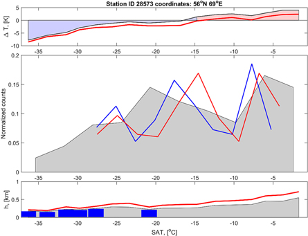
Figure 3. Histograms of the observed and modeled SAT from the same station as in figure 2. The SAT histograms are presented in the central panel. The gray bars present the observed SAT, the blue bars the SAT predicted with the old scheme and; the red bars— he SAT predicted with the new scheme. The curves and colors on the upper and lower panels denote the same quantities as in figure 2.
Download figure:
Standard image High-resolution imageContrary to common expectations, the new scheme does not improve the histogram at the low-SAT end, while it does introduce the improvements at the high-SAT end. The slopes of the dependences  on the upper panel are almost the same for the old and new schemes, but the new scheme produces smaller differences at higher temperatures. This behavior is surprising as the new scheme was sought to primarily improve the cold temperature prediction. Thus, the model with either scheme tends to over-predict not because it predicts systematically too high temperatures; in fact, the model under-predicts a high SAT, but because it does not reach the cold and warm temperatures during the cooling or warming events (see supplementary material). The major regular features found in the SAT errors remain in the analysis of all stations in both the European and Siberian regions (figure 4).
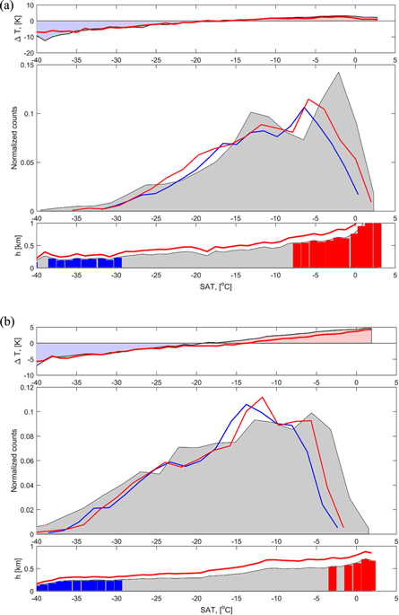
Figure 4. The same as in figure 3 but for all stations in the European (a) and Siberian (b) regions.
Download figure:
Standard image High-resolution image4.2. Analysis of the SAT tendencies
The observed systematic over-prediction,  of the lowest and under-prediction,
  of the highest temperatures suggests that the model produces SAT tendencies that are too small,
  As the surface heat budget over longer periods of time should be approximately correct in the model without systematic temperature drift, the damped tendencies indicate too large a scaling factor. Such a relationship between
  and
and  has been inferred from the solution in equation (2). We have also mentioned that this solution would have a low-pass filtering effect. It creates larger SAT differences under the action of higher-frequency forcing. Having enough data, we can statistically quantify this effect on the SAT.
The empirical histogram of  reveals that the larger tendencies are under-predicted in the model runs with both schemes (figure 5). Large positive skewness of 3.6 in the European and 2.8 in the Siberian regions indicates the presence of relatively short periods with strong warming tendencies. It is physically consistent with the advective nature of the winter-time warming events. Very large excess kurtosis (up to 11) points to a significant excess of large
  driven by persistent warming or cooling. At the same time, shorter (diurnal) heating does not produce large enough tendencies.
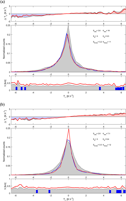
Figure 5. The same as in figure 3 but for the SAT tendencies taken from all stations in the European (a) and Siberian (b) regions.
Download figure:
Standard image High-resolution image4.3. Analysis of the SAT errors with respect to the ABL thickness
The ABL thickness was not identical in the forecast series with the old and new schemes. Although the new scheme does not modify  directly, it enhances the turbulent fluxes, and hence increases
  which is related to the mixing length scale through equation (3). Figure 5 and others show that
  in the new scheme is systematically larger than in the old scheme in all temperature and temperature tendency regimes. This gives us an opportunity to test the described effects of the scaling factor in equation (1) evaluating differences between these two forecasts.
The ABL thickness is larger in the forecasts with the new scheme. We divided the differences in the ABL thickness from these two forecasts into 20 bins. The SAT differences (errors),  were calculated for each bin of the
  differences. The analysis in figure 6 reveals that the new scheme indeed produces larger
  particularly in the western Siberian part of Russia. The SAT differences in the new scheme are smaller than those in the old scheme in all
  bins. One should note that 70% of the cases are found in the bins with the smallest
  differences of ±0.1 km where both schemes shows practically identical errors.

Figure 6. Dependence between the SAT errors,  in the old (blue) and new (red) schemes and the difference in the ABL thickness in these runs. The analysis is presented for the European (a) and Siberian (b) regions. The lines show the mean
  The bars show plus or minus one standard deviation for the data in each of 20 bins.
Download figure:
Standard image High-resolution imageWe further split  into five bins defined as
  < 0.25 km, 0.25 km < h < 0.5 km, 0.5 km < h < 0.75 km, 0.75 km < h < 1.0 km and h > 1.0 km. The ABL thickness is taken from the forecast with the old scheme. In each bin, the histogram analysis in figure 7 helps us to understand the internal statistical structure of the model errors. The model exhibits a robust positive difference in the runs with both the old and the new schemes. The difference is slightly less positive in the runs with the new scheme. However, the largest improvement caused by the new scheme is observed in the thickest ABL. In the Siberian region, the positive difference reduction by the new scheme is statistically significant for h > 0.75 km.

Figure 7. The model errors,  split in the five bins with the following
  thicknesses: <0.25 km, 0.25 <
  < 0.5 km, 0.5 <
  < 0.75 km, 0.75 <
  < 1.0 km and
  > 1.0 km. The European stations are shown in panel (a) and the Siberian ones in panel (b). Histograms of the model errors for each bin are shown by gray shading for the old scheme and by dashed lines for the new scheme. The mean
  and its standard deviations are shown by squares and vertical black lines. The mean values and numbers of 3-hourly observations in each bin are given on the plots. The histograms are normalized by their maximum values in each bin.
Download figure:
Standard image High-resolution image
5. Conclusions
Analysis of the energy-balance equation suggested that the temperature errors in the NWP forecasts could be equally sensitive to the model misrepresentation of the ABL thickness as to the misrepresentation of the surface energy budget and cloudiness. Previous studies reviewed in this paper have already indicated reciprocal relationships between the SAT errors and over-prediction of the ABL thickness in the reanalysis data and climate models. This study addressed the effects of ABL thickness on much shorter time scales of the diurnal forecast over northern Russia in the NWP model SL-AV of the HMCR.
The SAT errors in the ABL schemes are frequently considered in connection with the misrepresentation of the turbulent fluxes and their contribution to the surface energy budget. Repeated attempts to advance the turbulence parameterizations revisiting the flux schemes resulted in limited improvements of the forecast. The difficulties have been acknowledged in S13, BD14 and other publications. This study confirmed that the new TOUCANS (eeEFB) scheme demonstrates only limited advantages over the old (pTKE) scheme in the forecasts for the northern high-latitude regions. The new scheme reduced the SAT errors in the cases with a relatively thick ABL, partially because it made the ABL even thicker, but its performance in the cases with a shallow ABL remain problematic.
We propose a different perspective to relate the SAT errors and the ABL schemes. In previous modeling studies, the ABL thickness,  has not been treated as an independent prognostic parameter of the turbulence schemes. We disclosed that the SAT errors are organized in a consistent pattern relative to
  Two interconnected but distinct effects could be expected: (i) a large
  damps the magnitude of the SAT response corresponding to a given heat forcing; (ii) a large
  implies low-pass filtering on and reduces agility of the SAT response. The latter effect influences the modeled SAT tendencies, making the SAT differences larger in periods of high-frequency (e.g. diurnal) heat forcing fluctuations.
This consideration of  as an independent scaling factor suggests that the existing dependences between the turbulent fluxes and the mixing length scale in the ABL schemes should be relaxed. The original total turbulence energy theory in Zilitinkevich et al (2013) was built to account for the stability dependence of the turbulent Prandtl number, Pr. In a stratified atmosphere with a temperature inversion capping the ABL, this stability dependence of Pr implies that the turbulent fluxes may remain significant in a shallow ABL as well. This physics has been lost in the preparation of new ABL schemes. The suggested recovery of the independent
  treatment would not only be more adequate for modeling the physical nature of the ABL and the nature of
  as a scaling factor but should also add tuning flexibility to the model.
Acknowledgments
The study was supported by the Norwegian Research Council project no. 280573 'Advanced models and weather prediction in the Arctic: enhanced capacity from observations and polar process representations (ALERTNESS)'. The model forecast data and their analysis were produced at Hydrometcentre of Russia; this part of the study was supported with the Russian Science Foundation grant no. 14-37-00053P. The cooperation was supported by the Nordic Council of Ministers grant PECC TRAKT-2018.