

Abstract
Strong winter warming has dominated recent patterns of climate change along the Arctic Coastal Plain (ACP) of northern Alaska. The full impact of arctic winters may be best manifest by freshwater ice growth and the extent to which abundant shallow ACP lakes freeze solid with bedfast ice by the end of winter. For example, winter conditions of 2016–17 produced record low extents of bedfast ice across the ACP. In addition to high air temperatures, the causes varied from deep snow accumulation on the Barrow Peninsula to high late season rainfall and lake levels farther east on the ACP. In contrast, the previous winter of 2015–16 was also warm, but low snowpack and high winds caused relatively thick lake ice to develop and corresponding high extents of bedfast ice on the ACP. This recent comparison of extreme variation in lake ice responses between two adjacent regions and years in the context of long-term climate and ice records highlights the complexity associated with weather conditions and climate change in the Arctic. Recent observations of maximum ice thickness (MIT) compared to simulated MIT from Weather Research and Forcing (Polar-WRF) model output show greater departure toward thinner ice than predicted by models, underscoring this uncertainty and the need for sustained observations. Lake ice thickness and the extent of bedfast ice not only indicate the impact of arctic winters, but also directly affect sublake permafrost, winter water supply for industry, and overwinter habitat availability. Therefore, tracking freshwater ice responses provides a comprehensive picture of winter, as well as summer, weather conditions and climate change with implications to broader landscape, ecosystem, and resource responses in the Arctic.
Export citation and abstract BibTeX RIS
1. Introduction
Arctic climate is changing most rapidly during the early winter, particularly along coastal regions being impacted by declining autumn sea ice extents (Serreze and Barry 2011, Wendler et al 2014). The most striking change in climate during this season is increasing air temperature. For example, in the arctic coastal community of Utqiaġvik (formerly Barrow) in Alaska, mean annual air temperature (MAAT) increased by 1.5 °C from 1921–2012, with the most warming occurring in October—7.2 °C over the last 34 years (Wendler et al 2014) with additional record warm early winters of both 2016 and 2017 (table S1 is available online at stacks.iop.org/ERL/13/125001/mmedia). Changes in other components of the Arctic climate system, such as precipitation, wind intensity, storm events, and cloud cover, are often less apparent and subject to greater variability than temperature, but still important aspects of observed cold season climate change (Wendler et al 2014). It is sea ice decline interacting with these climate variables together that are causing notable responses in arctic landscapes and ecosystems and the plants, animals, and human communities that rely upon them (Post et al 2013).
The majority of physical and biological indicators currently being used to assess arctic climate change are thought to be responding to changes during the warm season (Oechel et al 1993, Chapin et al 2005, Overland and Wang 2013). Permafrost degradation in the form of coastline erosion (Jones et al 2009a), thermokarst (Jorgenson et al 2006, Kokelj and Jorgenson 2013), and active layer deepening (Shiklomanov et al 2010) are primarily considered to be in response to summer conditions. Trends in tundra greening and browning, vegetation productivity (Bhatt et al 2010, 2017), and shrubification (Tape et al 2006), and changes in plant and animal phenology (Post et al 2009) are also mostly considered in response to summer conditions. Spring responses such as snowmelt (Stone et al 2002, Cox et al 2017), river breakup (Tape et al 2016), and lake ice-out (Smejkalova et al 2017) timing capture portions of both cold and warm seasons. Declining sea ice in the Arctic Ocean is considered mainly in response to the summer melt season (Stroeve et al 2007), but creates a strong feedback with the Arctic climate system in the form of arctic amplification that spills over distinctly into winter (Serreze and Barry 2011), thus driving disproportionate changes during the cold season (Wendler et al 2014). Given the abundance of warm-season indicators, we are motivated to explore indicators of landscape and ecosystem responses to strong changes in winter that integrate multiple aspects of the climate system.
Perhaps the most obvious terrestrial landscape and ecosystem element of arctic coastal lowlands is the abundance of lakes and wetlands. For example on the Arctic Coastal Plain of northern Alaska (ACP), lakes cover greater than 20% of the land surface and wetlands cover up to another 50%–60%, which are mainly in the form of drained lakes basins (Hinkel et al 2005, Grosse et al 2013). Seasonal, freshwater ice forms in September or October and grows until May or June, historically reaching thicknesses of 2 m depending on winter temperature, but also in response to variation in snow depth and density and wind regimes (Zhang and Jeffries 2000). During warmer, often snowier, winters of the past decade however, end of winter maximum ice thickness (MIT) is often less than 1.5 m (Arp et al 2012). Variation in MIT cause shallow lakes to freeze solid in some years with bedfast ice and retain liquid water below floating ice in others (Zhang and Jeffries 2000). The extent of bedfast and floating ice on lakes can be readily tracked using satellite-based synthetic aperture radar (SAR) (Jeffries et al 1996). Multi-temporal SAR analysis of lakes on the Barrow Peninsula documents a dramatic shift in ice regimes from bedfast conditions to floating ice regimes (Surdu et al 2014). This lake ice regime shift documented on the Barrow Peninsula and other parts of the ACP is already impacting lake bed sediments and causing thawing of sublake permafrost (Arp et al 2016).
One of the major consequences of variable MIT is that sublake permafrost is typically stable under bedfast ice lakes compared to floating ice lakes where deep zones of thaw (taliks) exist in otherwise continuous permafrost (Burn 2002, Arp et al 2016). Floating ice lakes also support overwintering habitat for fish, can supply liquid water for building winter ice roads, and are less prone to summer drought (Arp et al 2015, Jones et al 2017). Climate model experiments demonstrate the role of sea ice decline in this lake ice response by isolating the effects of early winter warming and snowfall in the growth of lake ice (Alexeev et al 2016), but also underscore the complex role of snowfall amount and timing. An updated multitemporal SAR analysis for the Barrow Peninsula and other regions of Arctic Alaska in fact reveal very high interannual variability and more complex lake responses to winter climate than only considering air temperature would suggest (Engram et al 2018).
In this study, we focus on observations from the two recent winters on the ACP to demonstrate the complex responses among lakes, freshwater ice, and permafrost to winter climate. Lakes are increasingly recognized as indicators of climate change effects (Williamson et al 2009) and the lake-rich nature of arctic lowlands make lake interactions with climate and permafrost increasingly relevant (Grosse et al 2013). Observations of MIT and bedfast ice extent relative to air temperature, sea ice extent, precipitation, and wind regimes are considered for the winters of 2015–16 and 2016–17 relative to longer-term records. Contrasting lake ice responses in these two winters provide an example of how arctic freshwater ice observations, made in the field and by satellite, serve as excellent indicators of winter climate change with implications to broader landscape, ecosystem, and resource responses in the Arctic.
2. Methods
2.1. Study areas and monitoring networks
Monitoring of multiple lakes in Arctic Alaska began in the spring of 2012 as part of the Circum-Arctic Lake Observation Network (CALON, www.arcticlakes.org) and continued through the spring of 2018 as part of the Arctic Lake Ice System Science (ALISS, http://arcticlakeice.org) project. The objective of CALON was to collect data to understand patterns in lake physical processes across broad physio-climatic gradients (mountains to coastal plain) and within region scales of lake area and depth. Here we focus on two of the study nodes developed during CALON, Fish Creek and the Barrow Peninsula (figure 1(a)), to illustrate regionally contrasting responses in ice thickness and bedfast ice extent. Additionally, these two study areas have the benefit of long-term climate records from the National Weather Service station at Barrow, AK (station WBAN # 700260, WMO # 27502) and the US Geological Survey (Urban and Clow 2014) and Bureau of Land Management (Whitman et al 2011) in Fish Creek (table S1).
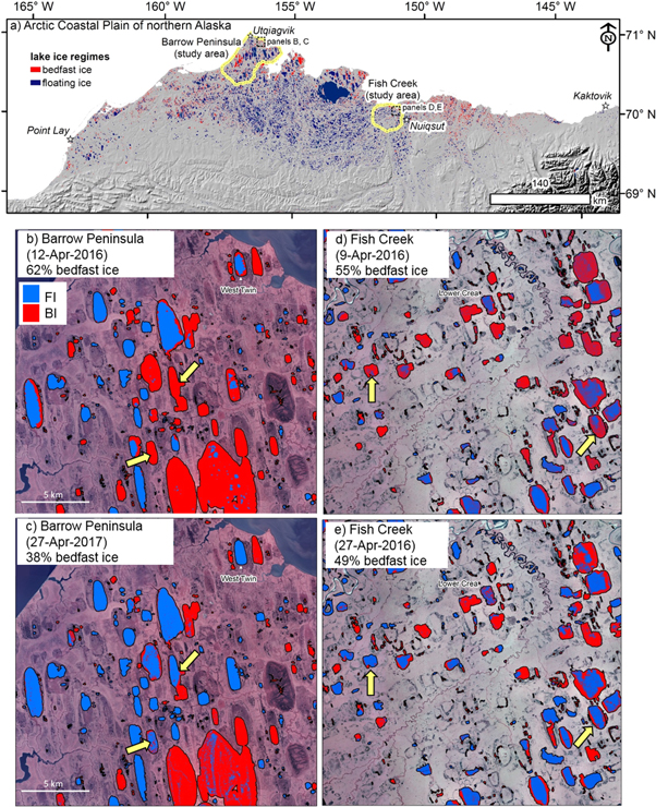
Figure 1. Map showing the location of two study areas on the Arctic Coastal Plain of northern Alaska and distribution of lakes classified by ice regime (A). Close-up views of focal lakes classified by bedfast (red) and floating (blue) conditions provide sharp contrasts between 2016 (B) and 2017 (C) on the Barrow Peninsula study area and these same years in the Fish Creek study area (D), (E). Yellow arrows indicate example lakes with major difference between years.
Download figure:
Standard image High-resolution imageAnalysis domains for the Fish Creek and Barrow Peninsula study areas correspond to a recently completed multi-temporal late winter SAR analysis from 1992–2016 (Engram et al 2018). In addition to providing comparable 25 year records of bedfast ice extent, this study also reports basic lake-centric landscape attributes and their variability. The Barrow Peninsula study area is located on the Outer ACP with 2228 lakes covering 23% of a 3067 km2 area. Many lakes in this study area are oriented NNW to SSE (Carson and Hussey 1962) and are of thermokarst origin with shallow bathymetry (<2 m depth) (Brewer 1958). Engram et al (2018) reported that 52% of the Barrow Peninsula lake area had bedfast ice averaged over a 25 year period. The Fish Creek study area is located on the Inner ACP with 1331 lakes covering 15% of a 1265 km2 area. Due to lower ice content permafrost in this region, lakes are not considered of 'true' thermokarst origin (Jorgenson and Shur 2007), though thermokarst processes result in lake expansion and a large portion of lakes are formed and shaped by fluvial processes as well (Jones et al 2017). Engram et al (2018) reported that 52% of the Fish Creek lake area had bedfast ice averaged over the same 25 year period. Both study areas lie in close proximity to the Arctic Sea coastline (figure 1(a)), yet the Barrow Peninsula juts out prominently into the Arctic Ocean with the Chukchi Sea to the west and the Beaufort Sea to the east, whereas Fish Creek lies adjacent to the Colville River delta that enters the Beaufort Sea at Harrison Bay.
2.2. Observations of maximum lake ice thickness
Records of lake ice thickness measured in late winter (mid-March to early May), when the ice is near its maximum thickness, have been made on the Barrow Peninsula since 1962. Many of these observations were made by the Alaska Lake Ice and Snow Observation Network (Morris and Jeffries 2010) and then the CALON and ALISS projects (Arp 2018). Similar records of late winter ice thickness have been made in the Fish Creek Watershed starting in 2006 in support of assessments of winter water supply for ice road construction in the National Petroleum Reserve in Alaska (NPR-A) and continued with the CALON and ALISS projects (Arp 2018). MIT is estimated from these late winter field observations by fitting lake ice growth curves simulated using a model based on Stefan's law (Lepparanta 1983), forced with air temperature and snow depth data on a daily time-step as described in greater detail in Arp (2018) and reported for shorter periods in Arp et al (2012). MIT is typically reached in late May to early June in most years when mean daily air temperature rises consistently above the freezing point. MIT is typically 5% thicker (5–10 cm) than observations made in April, on average, because ice grows very slowly during this late winter period.
2.3. Remote sensing of bedfast and floating lake ice
As described in Engram et al (2018), C-band SAR can be used to accurately determine lake ice regimes in shallow lakes because of the interaction of microwave energy with the physical properties of lake ice and ability to image at night and through dry snow to detect the presence or absence of liquid water below ice. In this study, we compared Sentinel-1 data acquired over the Barrow Peninsula on 12 April 2016 as reported in Engram et al (2018) and RADARSAT-2 data for Fish Creek acquired 9 April 2016 with a new Sentinel-1 image that covered both study areas on 27-April in 2017. April SAR scenes were selected to capture ice conditions as close as possible to MIT, but before the onset of spring melt, which typically occurs in mid-May, to avoid dampening the SAR signal from the presence of liquid water in melting snow or ponded on the ice surface.
SAR data processing and ice classification methods followed those of Engram et al (2018). Briefly, all data were first radiometrically calibrated, terrain corrected, and then geocoded to arrive at sigma-naught-scaled terrain-corrected GeoTiff files using the Sentinels Application Platform tool suite (v. 3.0) provided by the European Space Agency using elevation data from the Global Earth Topography And Sea Surface Elevation at 30 arc seconds (GETASSE30) dataset. We applied a Lee Sigma speckle filter (Lee 1981) in ERDAS Imagine (v2014), then manually checked and refined the geolocation accuracy of each image using a lateral translation where needed. Due to near-log normal characteristics of power-scaled SAR data (Dekker 1998), we performed a log-transform on the filtered radar intensity values resulting in data that were near-Gaussian distributed. Lake perimeters for each region, used to create a land-mask to isolate only the lake-ice pixels, were derived from IfSAR elevation data including use of Western ACP lake perimeters (Jones and Grosse 2013). A unique threshold for each SAR scene for each region was determined by utilizing the expectation-maximization (EM) approach, which assumed the bi-modal PDF of all lake-ice pixels was a mixture comprised of the bedfast ice pixel distribution and floating ice pixel distribution, both assumed to be Gaussian. The EM algorithm (Engram et al 2018) provides the means and variances of SAR σ0 for bedfast and floating ice classes as well as the unique threshold to delineate these lake ice regimes. The RADARSAT-2 Wide Ultra-Fine data for Fish Creek 2017 had a very high resolution, with small pixel (1.56 m) and large file sizes. Accordingly, we had to resample the pixel size to 3 m, resulting in a file size small enough to determine the bedfast/floating ice threshold with our EM algorithm, but we applied the resulting threshold to the original resolution image. Classification results from SAR data from different C-band platforms can be compared using an interactive threshold intensity for each SAR scene (Engram et al 2018). Both 2016 scenes and the 2017 scene were C-band single polarization (vertical-vertical) SAR.
3. Results and discussion
3.1. Lake ice in two contrasting winters and two arctic lowland regions
Field observations on the Barrow Peninsula in November of 2015 and 2016 provided an early indication of winter conditions in both years and associated lake ice growth response. Ice thickness measurements during these visits in mid-November and early December were used to estimate that ice was 81 cm thick on 1 December 2015 and 41 cm thick on the same date in 2016. For comparability, exact ice thickness on the same dates were estimated based on ice growth curves generated from the modified Stefan equation (Lepparanta 1983) and fit to observations made at slightly different times in each year (Alexeev et al 2016). Ice grows fast initially and gradually slows as a function of increasing ice thickness due to insulation from the overlying ice (Lepparanta 1983). Thus, these early measurements suggested that 2016 end-of-winter ice would be rather thick and 2017 end-of-winter ice would be rather thin. Differences in temperature are one explanation for these contrasting rates of ice growth—early winter (OND) air temperature averaged −15 °C in 2015, somewhat cooler than −10 °C observed in 2016.
Perhaps just as important as temperature in driving variation in lake ice growth between these years was the amount and distribution of snow we observed on lakes. In November 2015, snow cover on lakes averaged 6 cm depth and was drifted with many patches of bare ice. In November 2016, snow cover on lakes was only slightly deeper, averaging 10 cm depth, but was evenly distributed suggesting much less wind during and after snowfall events. Average wind speeds recorded at the Barrow NWS station were slightly higher during the winter of 2015–16, 6.6 m s−1, compared to 5.5 m s−1 in 2016–17. However, timing of strong wind events relative to snowfall events plays an important role (strong winds will blow new snow off the ice, as well as remobilizing existing snowpacks), although these quantities are very often difficult to decipher from station data. Measurements of snow depth on Barrow Peninsula lakes in late winter of 2016 averaged 20 cm and in late winter of 2017 averaged 29 cm. These differences in snow depth both in early and late winter between years may seem small, but the impact on ice growth between these amounts can be quite large (Zhang and Jeffries 2000, Alexeev et al 2016). Additionally, observations of the even snowpack in November 2016 suggests a greater stability and resistance to subsequent wind erosion and redistribution through the rest of winter. Conditions during snowmachine traverses in the early winters of 2015, very rough and slow traveling due to exposed tundra, compared to 2016, smooth and fast due to deeper and less drifted snow, were perhaps most telling as to the nature of the snowcovers' interactions with wind and were predictive of the eventual state of lake ice thickness we observed later in each of these winters.
Based on late winter (April) observations in both years, MIT reached 183 cm in 2016 and 120 cm in 2017 (figure 2(d))—3% higher and 33% lower, respectively, than the long-term average of 178 cm. Late winter SAR image analysis of the Barrow Peninsula showed that bedfast ice covered 62% of lake area in 2016 (figure 1(b)) and only covered 38% of lake area in 2017 (figures 1(c), 2(e)). This recent interannual variability in ice growth is striking for two reasons. One, the 183 cm thickness in 2016 is slightly higher than the long-term average despite a thinning trend over this period (Arp et al 2012, Surdu et al 2014). Whereas the MIT of 2017, 120 cm, is the lowest value we have on record for the Barrow Peninsula (figure 2(d)) (Arp 2018). Bedfast ice extent in 2017 was also the lowest on record since 1992 (figure 2(e)), when it averaged 51% of lake area (Engram et al 2018). Secondly, both winters were relatively warm overall, −17 °C and −15 °C, respectively, compared to the previous 28 year average of −20 °C (table S1). Temperature caused some difference in ice growth between these two recent years, but difference in snow cover and wind regimes likely were the more important factors causing contrasting interannual lake responses on the Barrow Peninsula.

Figure 2. Hierarchical time-series of linked oceanic and terrestrial hydroclimate datasets from sea ice (a), winter temperature (b), and late summer rainfall (c) that together drive ice thickness (d) and bedfast ice extent in the Barrow Peninsula (BP) and Fish Creek (FC) study areas. Focal winters of 2015–16 and 2016–17 are highlighted with dark gray and light gray bands, respectively.
Download figure:
Standard image High-resolution imageAn important lesson from multiple years of systematic measurements on Alaska's North Slope is that ice thickness and bedfast ice extent can show tremendous variability from one region to the next and these patterns are not necessarily consistent from year to year (Jones et al 2009b, Arp et al 2016). Comparing lakes in the Fish Creek Watershed, located ∼200 km to the SE and also along the Beaufort Sea coast (figure 1(a)), to the lakes of the Barrow Peninsula during the same two winters provides a nice example. At the Fish Creek lakes, MIT was 174 cm in 2016 and was 151 cm in 2017—slightly thicker to the same, respectively, as compared to the long-term record average, 150 cm, going back to 2003 (figure 2(d)). Winter air temperatures in the Fish Creek Watershed were similar between years, both −18 °C, and slightly warmer than the long-term average of −20 °C (table S1). Tundra snowpacks in both winters were slightly lower than the long-term average, explaining the somewhat thicker ice compared to temperature in both years.
This leads to another important lesson, and this one from satellite-based SAR analysis, is that bedfast ice extent does not always track MIT (Engram et al 2018) due to differences in water depth from year to year. Bedfast ice extent in April for the Fish Creek Watershed was also low in 2017, 49%, compared to 55% in 2016, despite MIT being relatively similar among years and actually thicker than the long-term average (figure 2(e)). This apparent disconnect between MIT and bedfast ice extent in some years most likely occurs because a lake's ice regime is controlled by ice thickness relative to lake depth. Typically water levels of thermokarst lakes are relatively stable from year to year, particularly during the late summer and early autumn when the influence of snowmelt is long gone (Arp et al 2011). However, rainfall totals at the Fish Creek watershed were much higher than normal in the late summer (August and September) of 2016, 89 mm, compared to the same period during the previous summer of 2015, 51 mm, and the longer-term average, 34 mm (figure 2(c)). The impact of this rainfall was apparent in several lakes in which water levels are regularly monitored, showing a late season rise of 16 cm (figure 3(b)), which likely was maintained going into freeze-up, such that lake depth increased relative to ice thickness during the ice growth season. Our late winter ice thickness surveys are always made at the same point (±10 m) of central lake locations each year and depth relative to the ice surface and water level are recorded. Water depth in Lake L9819 for example was 2.13 m in April 2017 compared to 1.93 m in April 2016. If similar lake level responses driven by abnormally high rainfall occurred throughout this region, this helps to explain our observations of exceptionally low bedfast ice extent despite average MIT at the end-of-winter 2017 (figures 1(e), 2(d), (e)).

Figure 3. Example two-dimensional (depth and time) depictions of lake ice growth and decay relative to lake depth over two winters for a lakes on the Barrow Peninsula (A) and Fish Creek (B) study areas.
Download figure:
Standard image High-resolution imageIn contrast to Fish Creek, where late-season rainfall explains low bedfast ice area, bedfast ice during the same years in the Barrow Peninsula region appears to be driven by lake ice processes. The late summer rainfall on the Barrow Peninsula in 2016 was approximately normal, 29 mm, compared to long-term average of 34 mm (figure 2(c)) and thus likely had little impact on lake levels. Late winter water depths recorded for focus lakes on the Barrow Peninsula confirmed similar levels as previous years when we have consistent measurements. Thus, the exceptionally low bedfast ice extent on the Barrow Peninsula was driven by record low MIT (figures 2(d), 3(a)). In both Barrow Peninsula and Fish Creek regions however, the impact of low bedfast ice extent would have the same effect on bed temperatures and sub-lake permafrost, as well as winter water supply and overwintering fish habitat (Arp et al 2016). Teasing apart these complex freshwater responses to winter weather and climate is made possible by using the combination of field-observed ice thickness and snow conditions, SAR ice regime analysis, and climate data.
3.2. Historic and future freshwater ecosystem responses to arctic winters
Reductions in autumn sea ice extent is seen as a major driver of winter climate change along arctic coastlines (Serreze and Barry 2011, Bintanja and Selten 2014). Longer and more extensive open-ocean waters not only cause warmer early winter temperatures, but also may be responsible for enhanced moisture delivery in the form of late summer rainfall and early winter snowfall (Liu et al 2012, Bintanja and Selten 2014, Alexeev et al 2016). All of these atmospheric responses being driven by sea ice dynamics can function to reduce growth of early winter lake ice. Perhaps not surprisingly, a positive correlation (r = +0.69) has been shown between September sea ice extent (Chukchi and Beaufort seas) and bedfast ice extent on lakes of the Barrow Peninsula in the following winter (Alexeev et al 2016). In this same study by Alexeev et al (2016) and highlighted by Brock (2016), the causal link between sea ice extent and lake ice growth has been demonstrated using a novel climate model experiment where 'high' and 'low' sea-ice extent years are interchanged with contrasting terrestrial climate years on the ACP of northern Alaska. Using Polar WRF to simulate these climate scenarios showed that 'ocean-effect snow' generated by greater open ocean was responsible for lower ice growth in the early winter and ultimately lower MIT and bedfast ice extent on freshwater lakes (Alexeev et al 2016).
Yet the impact of sea ice decline on early winter snowfall, air temperature, and freshwater ice growth also depends on storm tracks (Homan 2015), sea ice position relative to the coast (Alexeev et al 2016), whether precipitation falls as rain or snow, and the timing of snowfall relative to lake ice formation (Sturm and Liston 2003). In the case of the thick early and late winter lake ice observed in the winter of 2015–16, even though October sea ice extent was quite low overall, sea-ice concentrations were relatively high near the Barrow Peninsula (Alexeev et al 2016). This condition may have reduced early season snowfall locally, allowing more rapid ice growth. We observed relatively sparse snowcover on the tundra and lakes in November of 2015 with the additional impact of wind events that remove much of the snow that was initially deposited on lake ice surfaces. A more contrasting scenario for generating very slow ice growth likely occurred in the early winter of 2016, when sea ice was farther away from the Barrow Peninsula, air temperatures remained warm much longer into the early winter, and lake ice cover developed late. Once lake ice formed, steady snowfall in low wind conditions allowed a relatively thick and evenly distributed snowpack to accumulate and stabilize on lake ice, thus reducing lake ice growth for the remaining cold season.
A perfect scenario for both low ice growth and low extent of bedfast ice would have been if high late summer rainfall occurred on the Barrow Peninsula to raise lake levels prior to freeze-up, thus expanding the effective depth (ice thickness minus lake depth) (Arp et al 2016). High rainfall did occur in the Fish Creek Watershed ∼200 km to the SE, but this area had more normal early winter temperatures and snowfall in 2016–17 (figure 3(b)). Such complex interactions help explain why lake ice responses to winter climate change show such high variability despite strong winter warming (Wendler et al 2014). The scenario of high late summer rainfall coupled with high early winter snowfall and warm temperatures, is perhaps increasingly likely with continued declines in sea ice extent along the Arctic coastline.
Currently lake ice growth models do a rather poor job of capturing such complexities, primarily because the exact forcing data for physics-based lake ice models are unavailable (Ashton 1989, Kirillin et al 2012). Records of snow accumulation and snow density on lake ice are most critical for accurate models. Using air temperature and snow depth data generated from Polar WRF based on historic reanalysis data (1951–2005) and future projections (2006–2100) under a RCP-8.5 scenario (Cai et al 2018), we modeled MIT for the reanalysis period and projection period (figure 4). For the hindcast period, modeled MIT compared well for 9 out of 12 years when observation data were available (figures 4 and 5 and table 1). However, MIT observations in 1966, 1967, and 1997 were 43 cm thinner, on average, than simulated MIT using our ice growth model and Polar WRF reanalysis data. A possible cause of this discrepancy is higher snow accumulation on lakes than reanalysis data represents, though comparison with NWS snow depth data form tundra stations (table S1) show generally good agreement. Another possible explanation is that observations from 1966 and 1967 were only made on one lake and in 1997 only from two lakes following a different protocol to what is currently used where 4–6 lakes are typically surveyed per region (i.e. the Barrow Peninsula, Arp 2018) and it is quite possible that fewer lakes were not representative of regional ice growth.

Figure 4. Observed maximum ice thickness (MIT) for lakes on the Barrow Peninsula (Arp 2018) compared to simulated historical and projected MIT based on ERA-WRF and Polar WRF climate data (Cai et al 2018) (* indicated preliminary MIT based on mid-April observations and typical end of winter ice growth rates).
Download figure:
Standard image High-resolution image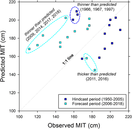
Figure 5. Maximum ice thickness (MIT) observed and predicted for hindcast and forecast periods as shown in figure 4 time series. Possible outliers during both periods are circled with years indicated.
Download figure:
Standard image High-resolution image
Table 1. Statistical summary of maximum ice thickness (MIT) data presented in figure 5.
| Hindcast period | Forecast period | |||
|---|---|---|---|---|
| Statistic | Observed | Predicted | Observed | Predicted |
| MIT mean (cm) | 187 | 187 | 153 | 179 |
| MIT standard deviation (cm) | 18.4 | 18.6 | 23.7 | 16.7 |
| Correlation coefficient (r) | −0.15 | 0.08 | ||
| p-value | 0.64 | 0.81 | ||
| Correlation coefficient (with outliers identified in figure 5 removed) | 0.75 | 0.94 | ||
| p-value | 0.02 | <0.01 | ||
Observations for the future projection period (2006 to present) are only expected to follow the mean trend for these 11 years. Yet three of these years, 2014, 2017, and 2018, fall well below, and two of these years, 2011 and 2016, are well above the modeled range of variability (figures 4 and 5). Comparison of model performance in these years indicate that the inability to represent snow depth on lakes, which is strongly subject to wind redistribution, is the primary factor in model predictions deviating strongly from observations. What is most striking is that such low MIT are not predicted by our climate-forced ice growth model until after 2040, which corresponds to the projected disappearance of perennial arctic sea ice in climate models (Cai et al 2018). The observed MIT values of 128 and 120 cm in two recent years are not consistently forecast by the climate-forced ice growth models until the last decade of our simulation between 2090 and 2100 when MIT averages 124 cm. Whether recent observations are an anomaly or a striking deviation from expected patterns of long-term, but gradual decrease in lake ice growth, this result points to high vulnerability to change and warrants future monitoring and consideration. Improvement of arctic climate models to capture sea ice interactions with snowfall and the wind redistribution of snow on lake surfaces would aid greatly in better performance of ice growth models in the future.
Field observations in April 2018 showed an average ice thickness of 105 cm on Barrow Peninsula lakes, but cannot yet be used to calculate an exact MIT because the ice growth season is still in progress. Comparison of past April observations with eventual MIT reached in late May suggest that the winter of 2017–18 will again break another record for thin ice on the Barrow Peninsula—we estimated a MIT of 111 cm based on previous records (figure 4). Three record low observations in 5 years are tempered by thicker than average ice observed in 2016. Thus, recent observations suggest strong deviation toward much thinner MIT than predicted, but also increased inter-annual variability, making predictions extremely challenging and necessitating dedicated observation programs to understand arctic freshwater ice dynamics.
4. Implications and recommendations
Our comparisons of lake ice conditions according to MIT and bedfast ice extent between two recent and contrasting years and two lake-rich regions of the ACP of northern Alaska demonstrate the complexities of freshwater ice responses to ongoing arctic climate change. MIT integrates winter climate in terms of air temperature relative to snowfall and wind conditions. MIT should also serve as a proxy for winter permafrost temperature regimes and freeze-back of the active layer (Jafarov et al 2014), although snowcover on lakes vs. the tundra can often be quite different from year to year (Sturm and Liston 2003). Bedfast ice extent is responsive to MIT, but also to variation in lake water levels that are controlled by late summer precipitation. In terms of broader ecosystem and societal impacts, changing ice regimes have implications for sub-lake permafrost stability and carbon stored in shallow sub-lake permafrost (Walter Anthony et al 2018). Reduced extents of bedfast ice in regions of the ACP where traditionally most lakes froze solid by the end of winter may cause widespread permafrost degradation, increased thaw subsidence and lake deepening, and the crossing of a permanent regime shift towards floating ice conditions (Arp et al 2016). Increased overwintering fish habitat and availability of liquid water for municipalities and winter ice road constructions may be considered positive impacts of this regime shift.
The link between thinner lake ice at MIT to sea ice decline comes in the form of warmer early winter air temperatures and in many cases higher snowfall during the early winter, which reduces lake ice growth (Alexeev et al 2016). However, depending on storm tracks and air temperature, early winter precipitation in the form of rainfall complicates this feedback. Even more confounding in terms of lake ice regime shifts, is the potential for enhanced moisture delivery from increasing and warmer open-water extent with reduced autumn sea ice extent. Observations from lakes in the Fish Creek study area show a very similar response in bedfast ice extent due to elevated lake levels. If ice thickness in 2017 in this area would have been similar to that observed on the Barrow Peninsula or conversely rainfall had elevated lake levels on the Barrow Peninsula in 2017 like they did in the Fish Creek area, then in both cases bedfast ice extents would have been reduced even further from what we observed. The potential for such circumstances would seem to be increasingly likely in future years if autumn sea ice extents continue to decline as anticipated (Massonnet et al 2012, Overland and Wang 2013).
Because freshwater ice and water balance are expected to respond in complex combinations to changing arctic climate and ocean conditions, the need for robust and dedicated observation strategies are warranted. Essential climate variables (ECVs) provide empirical evidence needed to understand and predict the evolution of climate, to guide mitigation and adaptation, assess risks and attribution of causes, and underpin climate services (Bojinski et al 2014). Accordingly, freshwater ice in the arctic landscape has been proposed as an ECV because it provides an integrative assessment of winter climate change and has wide ranging impacts on permafrost, carbon balance, water resource, aquatic habitat, and subsistence resources and transportation infrastructure (Engram et al 2018). The combination of remotely sensed bedfast ice extent, coupled with field observations of ice thickness together with standard weather station data provide the salient information to assess changing ice in lake-rich regions. Remote sensing techniques when combined with field observations increasingly provide useful information for understanding and adapting to environmental variability and change in the Arctic.
Acknowledgments
Funding for this study was provided primarily by the National Science Foundation (ARC-1107481, ARC-1417300) with additional funding from the US Geological Survey Alaska Science Center, the Arctic Landscape Conservation Cooperative, and the Bureau of Land Management Arctic Field Office. We thank B Gaglioti, G Grosse, and M Whitman who assisted with field work and logistics for this study. Two anonymous reviewers provided thoughtful input that improved this manuscript. Additional logistical support was provided by the staff from CH2MHill Polar Field Services, Inc. and Ukpeaġvik Iñupiat Corporation Science. We also thank O Ajadi for use of Matlab EM algorithm code. The majority of data used in this analysis are publically available at the Arctic Data Center at University of Santa Barbara.