

Abstract
Wind is a key component of the urban climate due to its relevance for ventilation of air pollution and urban heat, wind nuisance, as well as for urban wind energy engineering. These winds are governed by the dynamics of the atmosphere closest to the surface, the atmospheric boundary layer (ABL). Making use of a conceptual bulk model of the ABL, we find that for certain atmospheric conditions the boundary-layer mean wind speed in a city can surprisingly be higher than its rural counterpart, despite the higher roughness of cities. This urban wind island effect (UWI) prevails in the afternoon, and appears to be caused by a combination of differences in ABL growth, surface roughness and the ageostrophic wind, between city and countryside. Enhanced turbulence in the urban area deepens the ABL, and effectively mixes momentum into the ABL from aloft. Furthermore, the oscillation of the wind around the geostrophic equilibrium, caused by the rotation of the Earth, can create episodes where the urban boundary-layer mean wind speed is higher than the rural wind. By altering the surface properties within the bulk model, the sensitivity of the UWI to urban morphology is studied for the 10 urban local climate zones (LCZs). These LCZs classify neighbourhoods in terms of building height, vegetation cover etc, and represent urban morphology regardless of culture or location. The ideal circumstances for the UWI to occur are a deeper initial urban boundary-layer than in the countryside, low-rise buildings (up to 12 m) and a moderate geostrophic wind (∼5 m s−1). The UWI phenomenon challenges the commonly held perception that urban wind is usually reduced due to drag processes. Understanding the UWI can become vital to accurately model urban air pollution, quantify urban wind energy potential or create accurate background conditions for urban computational fluid dynamics models.
Export citation and abstract BibTeX RIS

Original content from this work may be used under the terms of the Creative Commons Attribution 3.0 licence. Any further distribution of this work must maintain attribution to the author(s) and the title of the work, journal citation and DOI.
1. Introduction
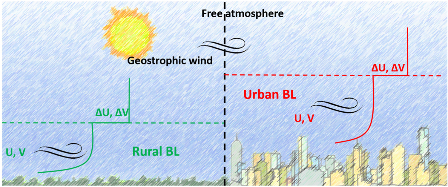
The heterogeneous landscape of (large) cities causes a complex micro-climate, which can vary from street to street. The combination of ongoing urban expansion and climate change underlines the need to understand the dynamics behind this microclimate. The urban microclimate directly impacts citizen health through additional heat [1], air pollution [2], and influences energy demand [3]. While urban heat has been widely studied [1, 4–6], knowledge about urban wind and its variability remains scarce [7, 8]. These winds are governed by the dynamics of the atmospheric layer closest to the surface, i.e. the atmospheric boundary layer (ABL) (figure 1).
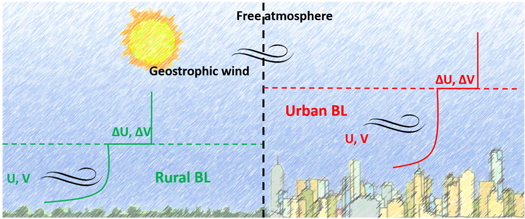
Figure 1. Schematic overview of the model. The rural column is indicated in green; the urban column in red. The dashed line represents the boundary-layer depth; U, V and ΔU, ΔV refer to the zonal and meridional wind, and their respective jumps to the geostrophic wind.
Download figure:
Standard image High-resolution imageThis study aims to quantify the difference in wind dynamics between city and countryside, using the conceptual mixed-layer model for the daytime ABL [9–12]. Urban wind has hitherto mainly been studied for individual buildings or street canyons [13], or over limited areas using computational fluid dynamics (CFD) models [8, 14, 15], though CFD models are increasingly able to model larger urban areas [16]. However, knowledge regarding mean wind behaviour at the scale of the ABL can be valuable for more general aspects, such as the mean wind load on buildings, wind potential for energy production [17] or wind nuisance in urban planning.
Differences between urban and rural wind dynamics can be caused by increased roughness, by enhanced surface heating due to the urban heat island (UHI) and changed ABL evolution. We aim to identify and understand these differences in wind behaviour through simulating contrasting wind regimes, by altering the surface parameters (roughness, displacement height, built fraction) and the initial conditions forcing the model (wind profile, geostrophic wind speed, boundary-layer depth).
Theeuwes et al [18] have used the mixed-layer model to show that for certain conditions, boundary-layer dynamics can explain the urban cool island: a period during the day where the city is colder than the countryside. Being aware of the impact of ABL dynamics, we hypothesize that an urban wind island (UWI), where the urban wind speed is larger than the rural wind speed, might form under favourable conditions.
2. Methodology
We use the conceptual mixed-layer model with a separated rural and urban column, as in Theeuwes et al [18]. We expand their model set-up with the bulk equations for the zonal (U) and meridional (V) wind components (figure 1).
2.1. Model description
The mixed-layer model is a slab model describing the mean ABL state. The model predicts well-mixed vertical profiles of turbulent quantities (heat, moisture, momentum), topped with a sharp jump (ΔU, Δ Θ, etc) to the free tropospheric profile, as well as the evolution of the ABL-depth (h). These conditions represent the convective daytime ABL, which is relevant when studying wind in the urban atmosphere. The tendency of the boundary-layer quantities is governed by their respective surface flux, and the entrainment flux, which mixes quantities down into the ABL from the troposphere and vice versa. Neither advection nor horizontal heterogeneity is considered. The simplified representation of the convective boundary layer makes these models very suitable for a wide range of conceptual studies [10–12, 19–21].
The mixed-layer equations governing the wind budget are:
Here U
geo
is the zonal
boundary-layer (geostrophic) wind;
V
geo
the meridional
boundary-layer (geostrophic) wind (all in m s−1);  and
and  are the surface and entrainment momentum fluxes (m2
s−2), respectively; h is the ABL
depth (m); f is the Coriolis-parameter taken at
10−4 s−1, representing mid-latitudes. A
full set of governing equations is presented in the supporting material of this
paper available online at stacks.iop.org/ERL/13/094007/mmedia.
are the surface and entrainment momentum fluxes (m2
s−2), respectively; h is the ABL
depth (m); f is the Coriolis-parameter taken at
10−4 s−1, representing mid-latitudes. A
full set of governing equations is presented in the supporting material of this
paper available online at stacks.iop.org/ERL/13/094007/mmedia.
2.2. Surface model
The model consists of two, non-communicating columns: an urban column and a rural column (figure 1). The columns are uncoupled to capture the behaviour of the urban effect on its own, rather than looking at rural-to-urban interactions (advection). The urban column represents a large metropolitan area, uninfluenced by the rural surrounding on the diurnal time-scale we are interested in. To distinguish between the urban and rural parts, underlying surface model parameters vary (e.g. the displacement height d is 0 m in the rural area, but significant in the urban area). The surface model contains a well-validated land-surface parametrisation valid for clear-sky, daytime cases [18]. The urban surface includes the effect of energy storage in impervious surface by using the objective hysteresis model [22] which calculates the storage heat flux from the net radiation and the urban building fractions.
2.3. Model validation
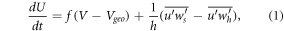
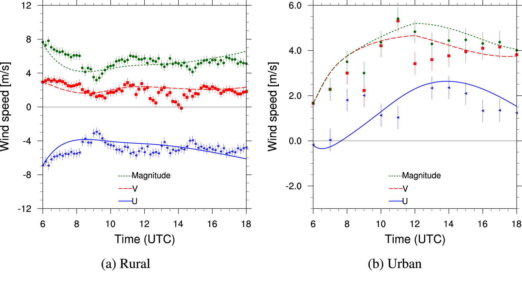
The rural part of the model is validated against observations from the Cabauw research tower, which measures the profile of wind speed among other quantities up to a height of 180 m. The Cabauw measurement site is a grassy field with a roughness length z0 of approximately 0.2 m, and few other roughness elements in its direct neighbourhood, which represents a typical rural field area [23]. Since the mixed-layer model is only valid for clear-sky, convective conditions, a set of clear days was chosen from the EUCAARIE campaign conducted in Cabauw in May 2008 [24] for model evaluation. We evaluate the modelled wind against the vertically averaged, layer-weighted wind observations between 10 and 180 m conform the bulk character of the model results. Geostrophic wind forcing is determined from surface pressure observations in a radius of 100 km around Cabauw.
The selected validation case is 4 May 2008, a clear-sky day with moderate wind speeds (geostrophic wind components Ugeo and Vgeo were on average −5 and +4.5 m s−1, respectively). The model simulation starts at 6:00 UTC (about 2 h after sunrise) and ends at 18:00 UTC (LT is UTC +2), to capture the full extent of the convective boundary-layer regime. The model captures the mean wind behaviour to a sufficient degree (figure 2(a)), though small-scale variability in the wind signal cannot be captured by the model due to its simplified physics and forcing. It seems the model produces relatively high friction in the first 2 h compared to the observations, visible by the sharp decline in the U and V wind components, which leads to an initial underestimation of the wind speed. Afterwards the model reproduces the measurements very well, though some low extremes in the V-component of the wind cannot be reproduced. Overall, the RMSE in the mean wind amounts to 0.8 m s−1 which is a robust result, given the simplifications within the model. Air temperature is modelled equally well, with an RMSE of 0.6 °C. The modelled surface energy balance (not shown) corresponds to observations, though the model initially underestimates the latent heat flux (by ∼40 W m−2), and slightly overestimates the sensible heat flux (∼15 W m−2) near the end of the model simulation.

Figure 2. Validation of the model, for (a) 4 May 2008 at the Cabauw observational site and (b) 23 July 2012 at the London King's College mast. Markers represent observations with error bars (10 min at Cabauw, 30 min at London); lines are the model outcomes. Green represents the wind magnitude (speed); in red and blue the meridional and zonal wind velocity components, respectively.
Download figure:
Standard image High-resolution imageThe urban part of the model is validated separately, against measurements taken at King's College, London, at 23 July 2012. Surface parameters are taken from [25], and forcing parameters (geostrophic wind, initial profiles) are taken from the SUBLIME case description for urban model intercomparison [26]. Observations are made on top of a building at 49 m above ground level (2.2 times mean building height), in a compact mid-rise neighbourhood. The chosen day is a clear-sky, convective day, though with substantial advection of momentum and a turning of the geostrophic wind with time, which we apply from SUBLIME.
The model performs satisfactorily (figure 2(b)), with an RMSE of 0.78 m s−1 for the mean wind speed. The model does not simulate the sudden jumps in wind speed seen in the observations, which can be attributed to the relatively low height of the observations, which still induces some turbulent behaviour from the street canyons below. The overall result is good, and the model can therefore be used with confidence to model both urban and rural mean wind speed.
2.4. Experiments
Having validated the model, we follow [18] for the model initialization, using initial values from the BUBBLE campaign in Basel (Switzerland) [27]. During this campaign 3 masts measured wind speed in and outside of Basel for an intensive observation period of one month. Since most of the urban measurements actually took place inside the urban canopy and roughness sublayer (below ∼2 times rooftop level [7]) which causes a lot of disturbance, direct validation of the urban wind is challenging. Hence we use the BUBBLE measurements to provide a typical urban–rural contrast at the start of the model simulation. This set-up is then used as a base run, against which further setups of the model are compared.
Considering the budget equations for momentum (equations (1) and (2)), the modelled wind is
influenced by three processes. The first process,
f(V − Vgeo
),
is the ageostrophic term, which redistributes momentum between the
U and V components of the wind, due to the
Earth's rotation. It follows that if
(V − Vgeo
)
(or
(U − Ugeo
))
is large,  has to increase as well. The second and third processes are in
the momentum flux divergence term, which contains a surface effect (
has to increase as well. The second and third processes are in
the momentum flux divergence term, which contains a surface effect ( ) and an entrainment effect (in
  ). When the fluxes are of equal sign, the momentum distribution
term is small and the ageostrophic term will dominate the momentum budget. When
the fluxes are of opposite sign, the momentum distribution term increases and
contributes more to the momentum budget. To determine which of these three
effects (surface, entrainment, ageostrophic) is dominant in determining
urban–rural wind contrasts, we perform a set of experiments.
). When the fluxes are of equal sign, the momentum distribution
term is small and the ageostrophic term will dominate the momentum budget. When
the fluxes are of opposite sign, the momentum distribution term increases and
contributes more to the momentum budget. To determine which of these three
effects (surface, entrainment, ageostrophic) is dominant in determining
urban–rural wind contrasts, we perform a set of experiments.
- 1.In the first experiment we eliminate the effect of the different urban surface. By setting the urban roughness lengths for heat and momentum to those of the rural surface, any influence caused by the buildings in a city is removed.
- 2.In the second experiment the entrainment rate is set to zero, to simulate a boundary-layer evolution without entrainment or detrainment from the free troposphere. The momentum budget is thereby only governed by the surface flux and the ageostrophic term.
- 3.The third experiment is to set the Coriolis parameter f to 0, which eliminates the ageostrophic term from equation (1), so only the momentum divergence plays a role. Though
 is not 0 in this case, but just leaves the
horizontal pressure gradient, we assume this to be negligible in
order to investigate the importance of the ageostrophic term as a
whole.
is not 0 in this case, but just leaves the
horizontal pressure gradient, we assume this to be negligible in
order to investigate the importance of the ageostrophic term as a
whole.

Finally, the 10 urban local climate zones (LCZs) ([28]) are implemented in the urban surface model, to study the influence of the urban fabric on the wind behaviour. Building height (and thereby displacement height and roughness length), urban and vegetation fractions are varied between these LCZs to simulate varying degrees of urbanization and urban morphology, and their respective effects on the wind.
3. Results
3.1. Reference case study
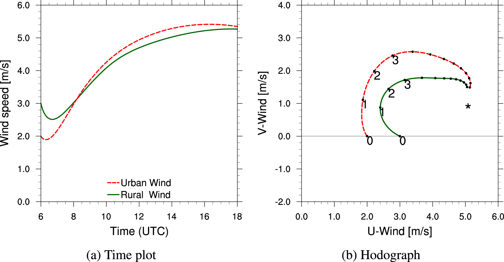
The urban model set-up resembles the city of Basel to represent the conditions of the BUBBLE campaign [27]. The geostrophic wind is set at 5 and 1 m s−1 for Ugeo and Vgeo , respectively, based on a climatology of the wind at sounding station Payerne (WMO code 06610) for June 2002 (the period of the BUBBLE campaign). Initial values of relevant model variables are given in table 1.
Table 1. Initial values of the model variables.  is the roughness length for momentum;
θ is the potential temperature.
is the roughness length for momentum;
θ is the potential temperature.
| Parameter | Urban | Rural |
|---|---|---|

| 1.5 m | 0.2 m |
| h | 400 m | 100 m |
| U(0) | 2 m s−1 | 3 m s−1 |
| V(0) | 0 m s−1 | 0 m s−1 |
| θ(0) | 288 K | 287 K |
| ΔU(0) | 3 m s−1 | 2 m s−1 |
| ΔV(0) | 1 m s−1 | 1 m s−1 |
| Δθ(0) | 4 K | 5 K |
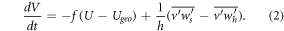
The model results for the reference case are depicted in figure 3. While the rural wind has a higher initial value than the urban wind speed, the urban wind speed accelerates for a longer amount of time after an initial drop at the start of the model run. This longer acceleration phase causes the urban wind to ultimately surpass the rural wind speed, creating a UWI at around 11 UTC, which reaches its maximum of 0.4 m s−1 at 14 UTC.
Figure 3. Model results for the reference case. In green are the rural model outcomes; urban in red. The asterisk in (b) indicates the geostrophic equilibrium wind, respectively; dots demarcate the hours (starting from 6 UTC). The numbers indicate the start of the model run (at 0) and the direction in which the hodograph should be read.
Download figure:
Standard image High-resolution imageAn interesting feature of this model run is visible in the hodograph (figure 3(b)). Both the urban and the rural wind show a clear inertial oscillation in time, moving clockwise around the geostrophic equilibrium wind vector. Such oscillations are typically associated with the stable nocturnal boundary layer [29–31], though several modelling and observational studies have also found these oscillations in the convective boundary layer (e.g. [11, 20]), where they significantly influence the wind, despite the effect of surface friction. Figure 3 shows that the rural oscillation seems to be more dampened than the urban oscillation, which describes a wider circle around the geostrophic equilibrium. This would suggest that either the rural part has a higher internal friction dampening the oscillation, or that the ageostrophic wind at the start of the model causes a larger amplitude of the urban oscillation. The larger amplitude of the urban oscillation causes the urban wind to accelerate for a longer period of time, thereby forming the UWI.
3.2. Experiments
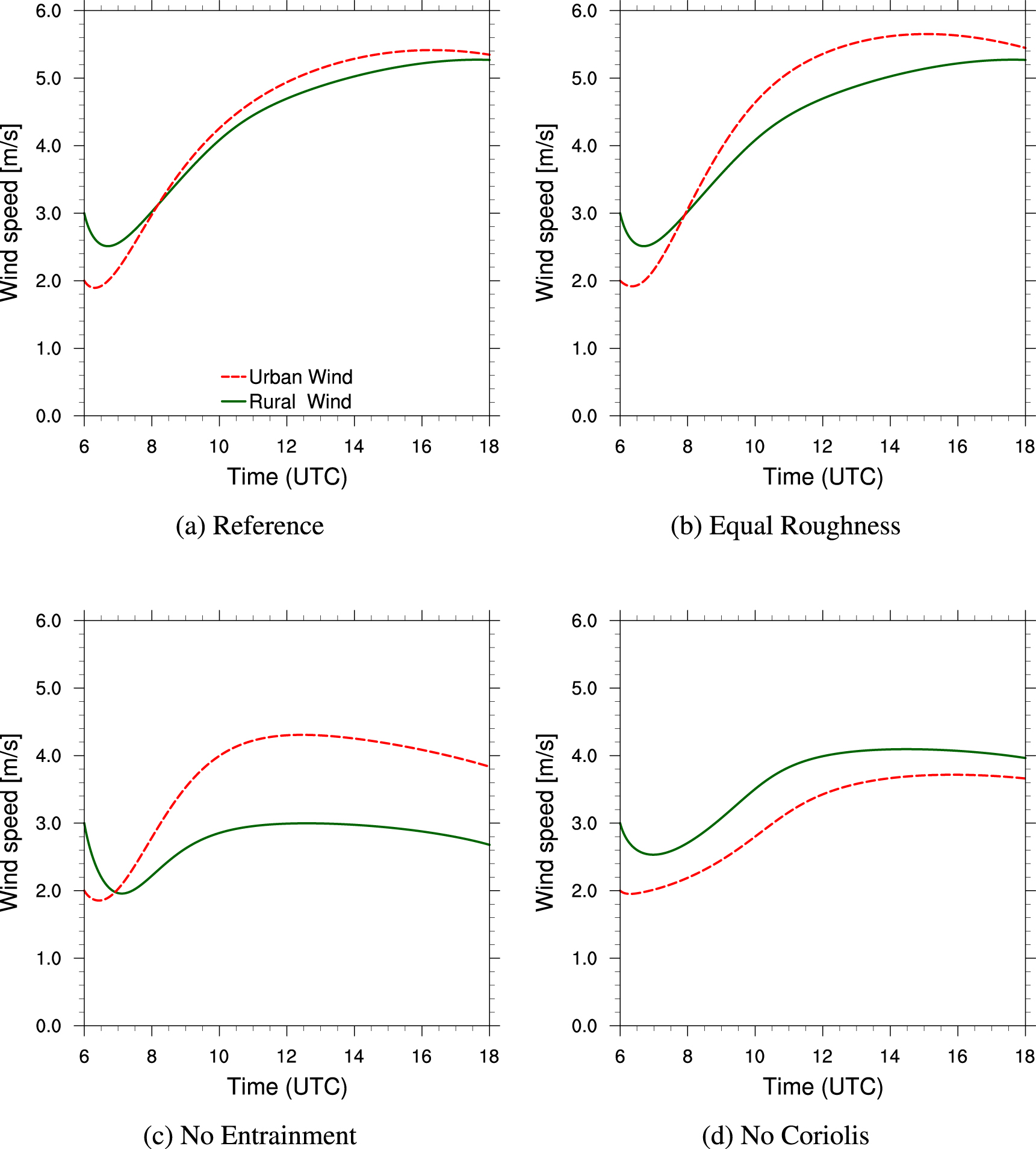
The experiments described in section 2.4 will focus on the UWI, and how the boundary-layer processes influence its modelled formation. Results of the first experiment, the equal roughness (figure 4(b)), are not very different from the reference run, though the urban wind values increase slightly. The urban surface momentum fluxes show a decrease, indicating lower friction generated by the surface, which causes the wind speeds to increase and enhances the UWI to ∼1 m s−1. Hence, roughness affects the UWI, but does not seem essential in its formation.
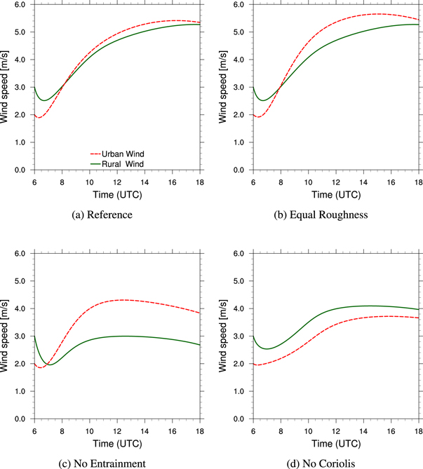
Figure 4. Modelled wind speed magnitude (m s−1) for (a) the reference case; (b) the equal roughness case; (c) the no entrainment case and (d) the no Coriolis force case. Urban wind is given in red; rural wind in green.
Download figure:
Standard image High-resolution imageThe second experiment, without the entrainment effect (figure 4(c)), shows remarkable differences between the urban and the rural response. Both the urban and rural wind become nearly stationary after 4 h, but the urban wind increases more rapidly, to ∼4.1 m s−1, whereas the rural wind initially decreases before slowly returning to its initial value (∼3 m s−1). The UWI is much larger than in the reference case (∼1.5 m s−1 versus ∼0.4 m s−1) due to the stationary rural wind. An analysis of the two components of equation (1) shows that the ageostrophic term and the momentum divergence term are nearly equal but of opposite sign after 4 h, effectively cancelling each other out. In the reference case the momentum divergence term is much weaker: this suggests that the entrainment counteracts against the surface flux, and that entrainment is an important source of momentum. To study whether the result of figure 4(c) is attributable to the entrainment, and not to the difference in initial boundary-layer height between urban and rural, we repeat the experiment with equal boundary-layer depths (shown in the supporting information). In this case, a UWI is not formed, indicating that the increased boundary-layer growth of the city plays a crucial role in reducing the impact of friction over the whole of the boundary layer.
Wind evolution is nearly stationary in the third experiment, (f = 0, figure 4(d)). Neither urban nor rural wind change much over the course of the model run, though the urban wind increases more than the rural wind. This indicates that the inertial oscillation is a key driver of the UWI, since a strong ageostrophic wind (f(V − Vgeo )) causes a stronger acceleration of the wind, and this ageostrophic wind will be higher for the cases where the urban wind is initially lower than the rural wind. The influence of the initial conditions of the model seems apparent here: with urban and rural wind speeds not evolving as dramatically as in the reference case, the initial conditions determine whether the UWI occurs or not (figure 4(d)).
3.3. Sensitivity to initial values and LCZs
The previous section revealed that the initial conditions are important contributors to the formation of the UWI. We examine the sensitivity for initial boundary-layer depth, wind speed, and geostrophic wind speed. In addition, we run the reference case for all 10 urban LCZs [28] to test how surface parameters such as roughness affect the model outcomes. For each sensitivity analysis, the model is run with the same settings as in table 1, with a range of values for the sensitivity parameter of interest. The sensitivity analysis is based on 11 values per parameter, linearly increasing between minimum and maximum values, for a total of 121 model runs per analysis. The wind-jumps range between 0--6.0 m s−1, and initial ABL depth from 50--400 m (rural) and 100--600 m (urban).
The modelled UWI formation appears to depend on the initial ageostrophic wind
(figure 5(a)). When the
ageostrophic wind of the urban area is large, the amplitude of wind oscillation
(as seen in section 3.2) becomes
larger and allows for a stronger UWI formation. Figure 5(b) shows the sensitivity of the modelled UWI to
the initial boundary-layer depth (h0) in the city and
countryside. The maximum UWI is found for those cases where the initial urban
boundary layer is several hundred metres higher than its rural counterpart. This
is likely linked to the boundary-layer dynamics as seen in section 3.2. The higher urban boundary
layer has a more efficient mixing, and smears out the surface friction over a
thicker boundary layer, decreasing  and
and  (equation (1)).
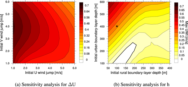
Figure 5. Sensitivity of the modelled UWI for the initial ΔU and ΔV (b) and boundary-layer depth (b). Contours indicate the value of the maximum (positive) UWI found, in m s−1. Model initialization for the other parameters is as in table 1. In (b) the asterisk denotes the values for the control case. Note that since U(0), V(0) are constant, the change in ΔU, ΔV changes Ugeo and Vgeo .
Download figure:
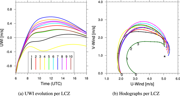
Standard image High-resolution imageThe effect of the urban surface on the UWI is further explored by implementing the surface characteristics of the 10 urban LCZs. Each LCZ has a distinct combination of properties such as building height and impervious fraction that alter the boundary-layer dynamics. The model is initialized with the reference case settings (given in table 1): the LCZ surface parameters are given in the supporting material, and more details of the LCZs in [28].
All but one LCZ show the UWI formation over the course of the model run, with the peak commonly around 12 UTC (figure 6(a)). LCZ 4 (open high-rise) does not show any UWI at all, though the similar LCZ in terms of building height, LCZ 1 (compact high-rise), shows a small UWI near the end of the model simulation (15 UTC). The building height for these LCZs is high (40 m), which in turn means that the displacement height is large. The increased friction causes a strong sink of momentum at the surface, which reduces the urban wind speed. The UWI formation in LCZ 1 can be attributed to the high urban fraction, which enhances the sensible heat flux, allowing for greater boundary-layer growth. This growth can enhance entrainment of momentum, and offset the strong friction at the surface by diluting the friction effect over a thicker boundary layer compared to LCZ 4, which is more open and therefore contains less high heat-storage material. The hodograph (figure 6(b)) shows the familiar oscillation for all LCZs, with few differences between LCZs. The weakest oscillation is seen in LCZ 1, where the wind is dampened by the strong surface friction.
Figure 6. Time evolution of the UWI for the 10 urban LCZs (a), and hodographs for the 10 LCZs and the rural area (b). The hodograph is similarly annotated as figure 3(b). LCZs 1 and 4 are high-rise, 2 and 5 are mid-rise, and 3 and 6 are low-rise classes.
Download figure:
Standard image High-resolution image
4. Discussion
4.1. UWI in previous studies
While there is a range of published urban wind studies, those that look at urban and rural wind differences are scarce, due to the difficulties in observing and modelling urban wind. Studies that take the broader scale of wind differences into account hint at the UWI phenomenon. Bornstein and Johnson [32] measure wind speed in and around the city of New York. For low wind conditions they find the urban wind, downwind of the city centre, can be increased with respect to the rural upwind values. They attribute this to the influence of the UHI, which causes enhanced turbulent flow. Other studies confirm these results, though the threshold below which the UWI varies per city and season. Chandler [33] and Lee [34] find a UWI for the city of London (England); Fortuniak et al [35] for Łódź in Poland; and Shreffler [36] for St Louis (United States).
The results of the first experiment in section 3.2 resemble the effect of the UHI, where enhanced mixing in the urban boundary layer can accelerate the wind speed. Using a two-dimensional mesoscale model, Byun and Arya [37] also model the differences between a rural and an urban site. Their results correspond to that of Bornstein and Johnson [32], Chandler [33] and Lee [34], as they also find a region of increased wind speed downwind of the city centre, attributed to the intensity of the UHI, but they do not directly relate its magnitude to that of the rural wind velocity. While our results are focused on the daytime wind behaviour with a conceptual model, both observations [32–36] and a more advanced mesoscale model [37] detect the UWI, and its formation due to the enhanced urban boundary-layer mixing. The strongest urban acceleration (UWI) occurs at night in most of these studies: however, Bornstein and Johnson [32] and Shreffler [36] also find a UWI during the weak daytime UHI with a similar magnitude as our results (∼0.5 m s−1).
4.2. Model choice
The model used in this study is a conceptual bulk model, which makes several assumptions to investigate a wide range of idealized wind conditions. However, an independent run of the single-column WRF model [38] (not shown) also displays a UWI with similar magnitude and timing, confirming the robustness of our applied model. The mixed-layer model only takes the mean boundary-layer wind into account, hence no vertical profiles of the wind can be modelled. In reality the boundary layer can experience vertical wind shear during neutral and weakly unstable conditions, especially in the complex terrain of cities [39–41], and knowledge of the vertical structure of wind speed is important for applications such as urban planning (e.g. through mechanical loads on buildings). Current models cannot easily simulate the flow field of wind inside an entire city: most limit themselves to either single buildings [42], homogenized canyons under various wind regimes [39] or rely on resource-intensive computation for an entire urban area [16]. Conceptual models can help improve understanding of the mean urban wind behaviour and be used to select interesting circumstances which a more sophisticated model can then study in more detail, in a limited area setting.
4.3. UWI
The UWI that we find seems to be caused by urban boundary-layer dynamics, but it stands to reason that wind differences can also be caused by specific rural boundary-layer dynamics. An example is the transition towards the stable boundary layer at the end of the afternoon, when surface heating dies down and buoyancy suppresses turbulence. This transition in the rural boundary layer will happen earlier than in the urban boundary layer, due to the UHI, caused by heat storage in the built-up surface [1, 22]. The nocturnal urban boundary layer often becomes neutral, where weak turbulence still produces (surface) winds, whereas the nocturnal rural boundary layer becomes stably stratified. The wind dying down in the rural area (before low-level jet formation) when there is still turbulence in the urban boundary layer, could potentially form a UWI. Observational studies [32–36] suggest an interplay between the UHI and the UWI, where a strong nocturnal UHI can fortify downward mixing of momentum into the urban boundary layer to further enhance the UWI. Whether this nocturnal UWI shares the same mechanisms with the afternoon-UWI that we find is a natural follow-up to this research. Rural-to-urban interactions of wind, such as urban breezes, are also not taken into account in this model, whereas they might play an important role in the horizontal distribution of momentum. We assume a decoupling between the urban and rural model parts, which in reality happens at distances of over ∼50 km, where the advection is small compared to the other components of the momentum budget. Using a 3D weather model could provide valuable insight in the daily cycle of the UWI, and how momentum is transported to create the UWI. Observations of the UWI are difficult to make, due to the strong influence of the urban canopy on the wind field, but at sufficient height (2–5 times building height [7]), tower measurements can be very useful for UWI detection.
5. Conclusions
Using a conceptual mixed-layer model of the urban and rural ABL we show that the mean wind in cities can exceed the wind in the rural surrounding. The model is validated against observations of the Cabauw tower facility in the Netherlands [23]. The model initial values and forcing are based on a climatology of the typical morning values measured in the BUBBLE campaign [27]. This UWI effect occurs primarily at the beginning of the afternoon, and has a magnitude typically around 0.5 m s−1. The UWI is caused by a combination of effects:
- 1.Enhanced mixing in the urban boundary layer which facilitates entrainment of free tropospheric air.
- 2.A deeper urban boundary layer that dilutes the increased urban roughness.
- 3.The imbalance between boundary-layer wind and the geostrophic wind, which accelerates the wind.
The initial model conditions also determine the magnitude of the UWI. Optimal conditions for the UWI are:
- 1.A deeper initial urban boundary layer than its rural counterpart.
- 2.A moderate initial wind speed and geostrophic wind speed.
- 3.Relatively low building heights (around 12 m).
An analysis of UWI magnitude for all 10 urban LCZs [28] reveals that the urban roughness from buildings decreases the UWI, and no UWI will form for high-rise LCZs. Insight in the UWI can be used to determine whether a city has potential for urban wind farming, and to provide background knowledge for more detailed studies, for instance in air quality modelling.
Acknowledgments
The authors acknowledge the CESAR database (www.cesar-database.nl) from which the Cabauw data was obtained, and would like to thank Fred Bosveld for supplying the geostrophic wind data. The authors thank Natalie Theeuwes for her help with the model development; Simone Kotthaus for supplying the urban data for London, and Aristofanes Tsiringakis for his help with the SUBLIME boundary values. AD and G-J S acknowledge funding from the Netherlands Organization for Scientific Research (NWO) VIDI Grant 'The Windy City' (file no. 864.14.007).