

Abstract
Hurricane Harvey brought to the Texas coast possibly the heaviest rain ever recorded in US history, which then caused flooding at unprecedented levels. Previous studies have shown that large arrays of hypothetical offshore wind farms can extract kinetic energy from a hurricane and thus reduce the wind and storm surge. This study quantitatively tests whether the hypothetical offshore turbines may also affect precipitation patterns. The Weather Research Forecast model is employed to model Harvey and the offshore wind farms are parameterized as elevated drag and turbulent kinetic energy sources. Model results indicate that the offshore wind farms have a strong impact on the distribution of accumulated precipitation, with an obvious decrease onshore downstream of the wind farms, and an increase in offshore areas, upstream of or within the wind farms. Compared with the control case with no wind turbines, increased horizontal wind divergence and lower vertical velocity are found where precipitation is reduced onshore, whereas increased horizontal wind convergence and higher vertical velocity occur upstream of or within the offshore wind farms. The sensitivity to the size of the offshore array, inter-turbine spacing, and the details of the wind farm parameterization are assessed. The results suggest that large arrays of offshore wind turbines can effectively protect the coast from heavy rain during hurricanes and that smart layouts with fewer turbines over smaller areas can be almost as effective as those with more turbines over larger areas.
Export citation and abstract BibTeX RIS

Original content from this work may be used under the terms of the Creative Commons Attribution 3.0 licence.
Any further distribution of this work must maintain attribution to the author(s) and the title of the work, journal citation and DOI.
1. Introduction
Wind farms provide clean electricity by extracting energy from the wind flow. Since the wind flow is affected during the energy conversion, it is expected that the disturbed wind flow can affect the environment and local weather, e.g. temperature and precipitation. Both numerical studies (Baidya Roy et al 2004, Adams and Keith 2007, Baidya Roy and Traiteur 2010, Wang and Prinn 2010, Somnath Baidya 2011, Fitch et al 2013, Lu and Porté-Agel 2015) and observations (Zhou et al 2012, Rajewski et al 2013, Smith et al 2013, Rajewski et al 2014) have found surface temperature changes in the presence of wind farms. However, very few studies have focused on the impact of wind farms on precipitation. A numerical study by Wang and Prinn (2010) found that large-scale installation of wind power may lead to alterations in global distributions of rainfall (10% in some areas). Another study (Fiedler and Bukovsky 2011) found that, although an onshore wind farm may have a strong impact on precipitation during one season, only a slight impact, not statistically significant, was detected over a 62-season average. A recent study (Possner and Caldeira 2017) modeled large-scale wind farms both in the open ocean and on land, and found no statistically significant changes in surface precipitation.
In this study, we assess whether a large, hypothetical array of offshore wind farms can inadvertently impact precipitation during severe weather conditions like hurricanes. In the literature, Jacobson et al (2014) have shown that offshore wind farms can reduce wind speed and storm surge during hurricanes, but did not assess the impact on precipitation. Fiedler and Bukovsky (2011) claimed that precipitation during a few tropical cyclones in the Gulf of Mexico was significantly altered by the presence of inland wind farms; however, the wind farms were far from the evaluated areas and the forecast accuracy of the simulations was not validated. Moreover, the simulation results were for a whole summer season, which is inadequate to prove that the impacts are mostly within tropical events (usually lasting a few days).
In this study, the case study of Hurricane Harvey is chosen since it brought to the Texas coast possibly the heaviest rainfall on record and caused severe flood damage to the metro-Houston areas. The effects on precipitation may be easier to detect with a large amount of rainfall, thus it is an ideal case to study precipitation. The Weather Research Forecast (WRF) model version 3.6 is employed to simulate Hurricane Harvey. The Advanced Research WRF version (ARW) is used instead of the hurricane version with data assimilation (HWRF). Although the latter has shown superior performance in previous studies of hurricanes (Dodla et al 2011), the goal of this study is not to simulate Hurricane Harvey perfectly, but rather to simulate the impacts of future offshore wind farms as realistically as possible. Assimilating observations that were collected in the absence of such wind farms would not be realistic in simulations that include wind farms, therefore ARW was run without data assimilation and without the complex data-driven vorticity enhancements used in HWRF. The simulation results without wind farms are validated with observations, including hurricane track, minimum sea level pressure, wind field and precipitation in Houston, in order to ensure a reasonably accurate forecast. The wind farms are modeled using the Fitch parameterization (Fitch et al 2012), which is the most widely used wind farm parameterization in mesoscale models. An additional case, which used the enhanced surface roughness method to represent the effects of wind farms, was also simulated to verify the sensitivity to wind farm parameterization.
2. Simulations
In this section, the details of the simulations and the validation against observations are presented.
2.1. Setup
The model domain is set up to cover the coast of Texas and Louisiana, as shown in figure 1. The horizontal resolution is Δx = Δy = 10.667 km. The initial and boundary condition data are taken from the North American Mesoscale Forecast System with a resolution of 12 km. The model is integrated for four days from 0000 UTC August 25, 2017 to 0000 UTC August 29, 2017 with a 6 hour spin-up. The 1.5-order, 2.5 level MYNN PBL scheme (Nakanishi and Niino 2009) is selected since the wind farm parameterization is dependent on this scheme and it is widely used in the literature (Fitch et al 2013, Volker et al 2015, Eriksson et al 2015). The Kain–Fritsch convective parameterization scheme (Kain and Fritsch 1992, Kain 2004) is used to predict the convective component of precipitation and the land-surface model is Noah (Ek et al 2003). The details of the simulation setup are presented in table 1.

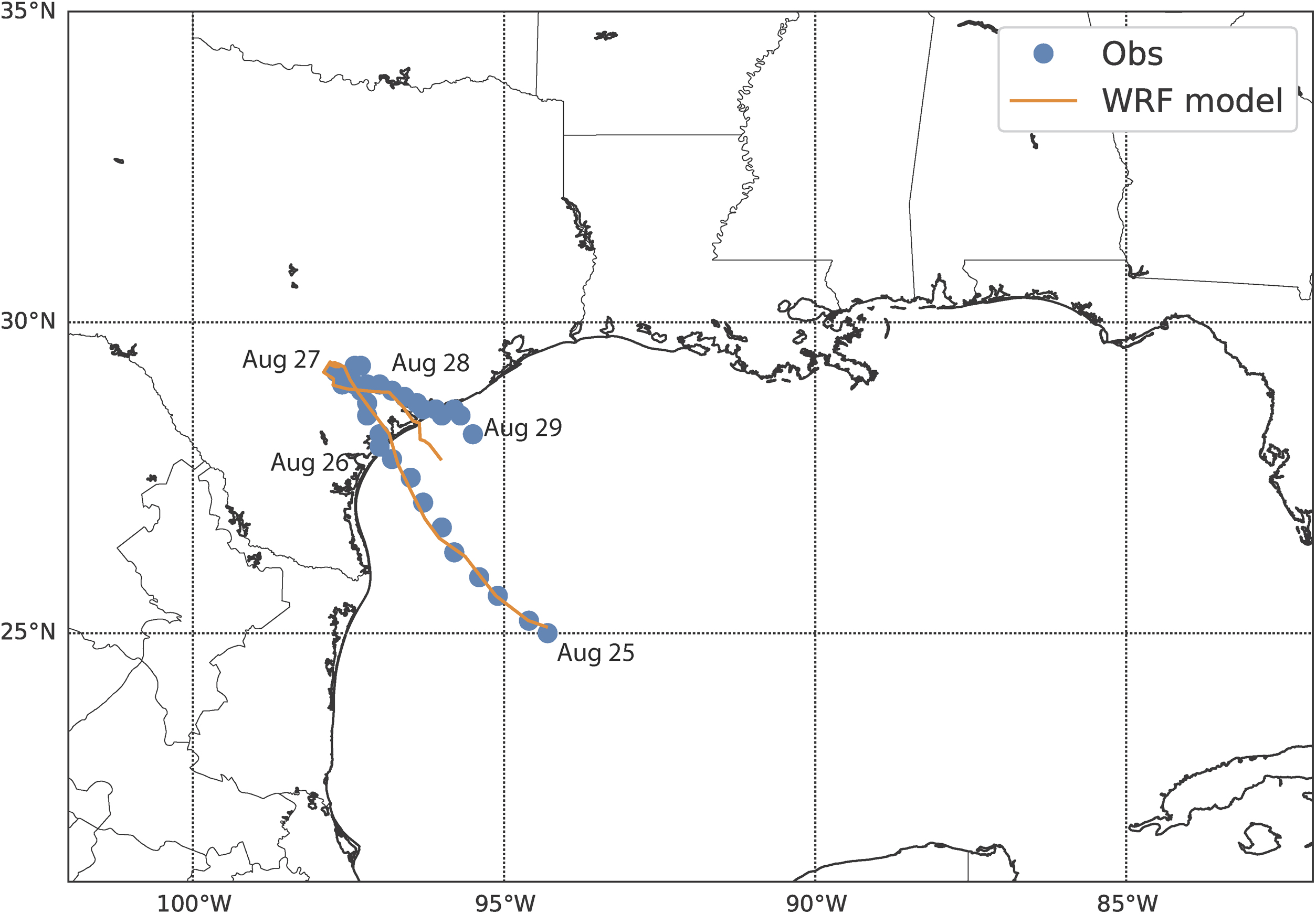
Figure 1. The model domain used in this study, with Hurricane Harvey's track from observations and from the CTRL simulation.
Download figure:
Standard image High-resolution imageThe wind farms are modeled using the Fitch wind farm parameterization (Fitch et al 2012), which models the wind farms as a momentum sink and an added turbulent kinetic energy (TKE) source. The magnitude of the drag force on the atmosphere induced by one wind turbine can be expressed as:
where V is the horizontal wind speed over the disk, CT is the thrust coefficient, ρ is the air density, and A is the disk area swept by the turbine rotor. The rate of loss of kinetic energy in the wind  is therefore:
The extracted kinetic energy in the wind goes into the electric power (via a power coefficient) and additional turbulent kinetic energy (via a TKE coefficient). The energy losses induced by heat via friction and mechanical losses are ignored. Note that the wind turbines in the Fitch parameterization correctly extract kinetic energy in a manner that depends on the thrust coefficient, which is a function of wind speed (CT (V)). As such, no energy is extracted at wind speeds below the cut-in or above the cut-out wind speeds, as real turbines do. If the wind at a grid cell reaches or surpasses the cut-out wind speed during a hurricane simulation, then the turbines are effectively shut down at that grid cell.
The other approach employed to parameterize the wind farms is to increase surface roughness, which was first introduced by Keith et al (2004). Although the surface roughness parameterization is overly-simplified, as wind turbines extract energy not near the surface, but rather around the rotor disk, it is computationally efficient and therefore has been used extensively in large-scale simulations of wind farms (Kirk-Davidoff and Keith 2008, Barrie and Kirk-Davidoff 2010, Wang and Prinn 2010, Miller et al 2011). In this study, the surface roughness parameterization is used to model a supplemental case for sensitivity purposes, aimed at demonstrating that the conclusions derived from our study are robust and do not depend on the exact implementation of the wind farm parameterization.
A control case with no wind farms, denoted as CTRL, is run first. The CTRL case is set up to ensure the accuracy of the simulations and highlight the precipitation differences induced by the turbines under the same model configurations. Five additional cases with different layouts are run next (details in table 2). For all cases, turbines are installed in waters up to 200 m in depth, due to the technical difficulty and high construction costs in deeper water areas. The wind turbine model is the 7.5-MW Enercon 126 with a diameter D = 126 m and cut-in and cut-out wind speeds of 3 and 34 m s−1 respectively. To study the best wind farm location, three basic cases (LWF, MWF, SWF for large, medium, and small wind farm), shown in figure 2, are modeled that cover differently sized offshore areas, but with the same inter-turbine spacing. Two additional cases cover the same areas as MWF, but with tight (MWF-TS) and wide (MWF-WS) inter-turbine spacings. For all the wind farm cases except SWF, all the turbines were placed along the coast, ranging from the coastline to 100 km offshore (including the bay areas). The SWF case is similar to the MWF case, but only the turbines within the commercial lease zone from the Bureau of Ocean Environment and Management (BOEM) are modeled, in order to avoid the non-construction areas and achieve a more realistic configuration. A supplemental case (MWF-Z0) is modeled with the same setup as MWF but with an increased surface roughness z0 = 0.5 m over the turbine areas. The surface roughness value was determined via a series of tests, as described later in section 3.2.
Table 1. Summary of the WRF model settings used in the simulations.
| Number of grid points | NX = 155, NY = 122, NZ = 41 |
| Horizontal grid spacing | 10.667 km |
| PBL scheme | MYNN |
| Surface layer scheme | MYNN |
| Land surface model | Noah |
| Cumulus scheme | Kain-Fritsch |
| Wind farm parameterization | Fitch |
Table 2. Summary of the simulation cases. D is the diameter of the wind turbine.
| Cases | No. of turbines | Location | Spacing |
|---|---|---|---|
| Control | 0 | N/A | N/A |
| LWF | 74 619 | Coast to 100 km | 9D × 9D |
| MWF | 33 363 | Coast to 100 km | 9D × 9D |
| SWF | 28 197 | Within BOEM lease zone | 9D × 9D |
| MWF-WS | 22 242 | Coast to 100 km | 11D × 11D |
| MWF-TS | 59 312 | Coast to 100 km | 7D × 7D |
| MWF-Z0 | N/A | Coast to 100 km | N/A |

Figure 2. Location of the wind farms in the three layout configurations: (a) LWF, (b) MWF, and (c) SWF. The difference between the layout of MWF and SWF is the strip with no turbines along the coast in SWF.
Download figure:
Standard image High-resolution image2.2. Validation
To ensure the accuracy of the simulations, with and without wind farms, the results of the CTRL case (without wind farms) are compared with the observations, including hurricane track, minimum sea level pressure, maximum wind speed, and precipitation. The precipitation data are provided by the Harris County Flood Warning System (2017), and other observations data are from the National Hurricane Center (NHC) accessed from The Weather Company (2017).
The simulated track of Hurricane Harvey agrees well with the observation data prior to August 29, 2017 and is slightly off afterwards (figure 1). Considering that the rainiest days for the metro-Houston area were before August 29, only the results of the first four days will be analyzed in this study. The time series of simulated maximum 10 m wind speed and minimum sea level pressure during the four days prior to August 29 show a good level of accuracy when compared against observations from NHC data, especially considering that no observations were assimilated into the simulation (figure 3). The modeled minimum sea level pressure (figure 3(b)) generally follows the trend of the observations, except for an underestimate at the time when the hurricane was strongest. However, the timing of the lowest minimum coincides almost perfectly with the observations.
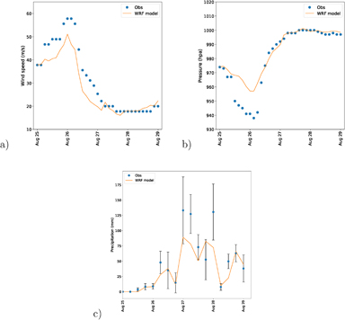
Figure 3. Comparison of the CTRL simulation results with observations during Hurricane Harvey: (a) maximum 10 m wind speed, (b) minimum sea level pressure, and (c) precipitation near downtown Houston.
Download figure:
Standard image High-resolution imageIn order to validate the precipitation predictions, simulated values were extracted at a grid point located downtown Houston from the model domain. Data from 15 gauges from Harris County Flood Warning System (2017) located within the downtown grid point were averaged to make the simulation results and observation data comparable. The simulation results generally underestimated precipitation (figure 3(c)), but most of the time the results are within the error bars. The timings of the two peaks between August 27 and 29 are both close to the observed. The discrepancy between the model results and the observations is possibly due to the lack of vortex initialization and data assimilation, which have been proven to improve the accuracy of the cyclone track and intensity (Kurihara et al 1995, Wang 1998, Cavallo et al 2013, Zhang et al 2009, Zhang et al 2011, Hamill et al 2011) but cannot be used for sensitivity runs as those conducted in this study. Although the magnitude of the prediction is slightly off from the observations, the general trend of the results matches. Thus, the CTRL results can be used as a reference state to further evaluate the impacts of the wind farms.
3. Results
3.1. Precipitation reduction due to horizontal divergence
The wind farm parameterization correctly extracts kinetic energy at the wind farm locations, as shown by the horizontal distribution of wind speed at hub height at 0900 UTC on August 25, 2017 (figure 4). For the same farm, the wind speed reductions depend on the density of turbines. For example, higher wind speed reductions (and therefore higher energy generation) are achieved in the MWF-TS than in the MWF or MWF-WS cases, due to the higher number of turbines (59 312 vs. 33 363 and 22 242, respectively).

Figure 4. Hub-height winds speed results at 0900 UTC August 25, 2017: (a) wind speed (m s−1) in CTRL case; and (b)–(f) wind speed difference (m s−1) between the cases indicated in the figure labels and CTRL.
Download figure:
Standard image High-resolution imageFrom figure 3(c), the largest precipitation amounts occurred during the last three days (August 26 to 29) and therefore this time period is selected for further analysis. Looking at 72 hour accumulated precipitation patterns (figure 5), both areas with increased precipitation and areas with reduced precipitation are found due to the presence of the wind farms, but not in a random manner. Rather, increased precipitation is found mostly offshore, upstream of or within the wind farms, while reduced precipitation is found onshore or close to the coastline, downstream of the wind farms. Considering the damage caused by precipitation and flooding in the metro-Houston area, this coherent pattern of reduced precipitation onshore suggests that huge potential benefits, in terms of avoided damage and lives saved, could be harnessed by installing large offshore wind farms in the Gulf.
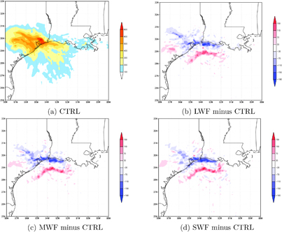
Figure 5. 72 hour accumulated precipitation (mm) or precipitation difference (mm) during 26–29 August 2017: (a) CTRL, (b) MWF minus CTRL, (c) LWF minus CTRL, and (d) SWF minus CTRL.
Download figure:
Standard image High-resolution imageCompared with the MWF case (figure 5(c)), the LWF case (figure 5(b)) produces very similar changes in precipitation patterns, especially along the coast near Houston, even though the latter covers a much larger area and has more than twice the number of wind turbines. The physical mechanisms behind this finding will be explained in the next paragraph, but for the moment it can be concluded that an array of wind farms as large as that in the LWF case is not necessary since it produces little improvement in the benefits with much higher costs than the MWF case. This is the reason that the sensitivity tests to inter-turbine spacings in section 3.2 will be based on the MWF case.
To better quantify the changes in precipitation, a sector covering south Houston (−95.7° W to −95.2° W and 29.5° N to 29.8° N) is selected for further analysis. The simulated precipitation amount is averaged over this sector. The reduction in the 72 hour accumulated precipitation (see table 3) is approximately 15% for both the MWF and LWF case. For the SWF case, the reduction is only about 10%, which suggests that the wind farms placed in the Galveston Bay areas, missing in SWF, could be of great importance for the city of Houston.
The hypothesis put forward here is that changes in precipitation—increases offshore and decreases onshore—are associated with changes in horizontal wind divergence and in vertical wind speed caused by the wind farms. To verify this hypothesis, the difference between these two terms in the LWF case minus the CTRL case at landfall are shown in figure 6. To the northeast of the hurricane center, the wind is blowing from the sea towards the land. In these areas, the horizontal wind divergence difference (LWF minus CTRL in figure 6(a) is negative upstream of the wind farms, as the wind slows down because of the presence of the wind farms, and is positive downstream of the wind farms, as the wind speed recovers past the wind farms. Correspondingly, the vertical wind speed difference (figure 6(b)) is positive upstream of the wind farms, meaning that upward motion is enhanced and therefore precipitation is increased, and negative downstream of the wind farms, meaning that upward motion is suppressed and therefore precipitation is reduced. To the south of the hurricane center, the wind is coming from the shore, so changes in the horizontal wind divergence and vertical wind speed are opposite to those to the northeast of the hurricane center. However, over the entire 3 day period, no substantial changes in precipitation were found in these areas.
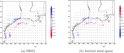
Figure 6. Results at hub height at landfall: (a) horizontal divergence difference (s−1) LWF minus CTRL, (b) vertical wind speed difference (m s−1) LWF minus CTRL.
Download figure:
Standard image High-resolution image3.2. Sensitivity analysis
To assess the sensitivity to inter-turbine spacing and parameterization formulation, the focus of this section will be on the 24 hour accumulated precipitation from 26 to 27 August 2017, during which the winds were strongest and the effects of the wind farms on precipitation were more pronounced (figure 5(c) vs. figure 7 (a)). From the 24 hour accumulated precipitation difference between the wind farm cases with various inter-turbine spacings and the MWF case with no wind turbines (figure 7), obvious precipitation reductions onshore can be noticed. The compact case (figure 7(b)), with more turbines than the MWF case (figure 7(a)), exhibits a stronger reduction in precipitation inland and a stronger increase in precipitation offshore and over larger areas. Vice versa, in the wide-spacing case MWF-WS (figure 7(c)), the precipitation changes are qualitatively the same, but smaller in magnitude and areal extent.

Figure 7. 24 hour accumulated precipitation difference (mm) from 26–27 August 2017: (a) MWF minus CTRL, (b) MWF-TS minus CTRL, (c) MWF-WS minus CTRL, (d) MWF-Z0 minus CTRL.
Download figure:
Standard image High-resolution image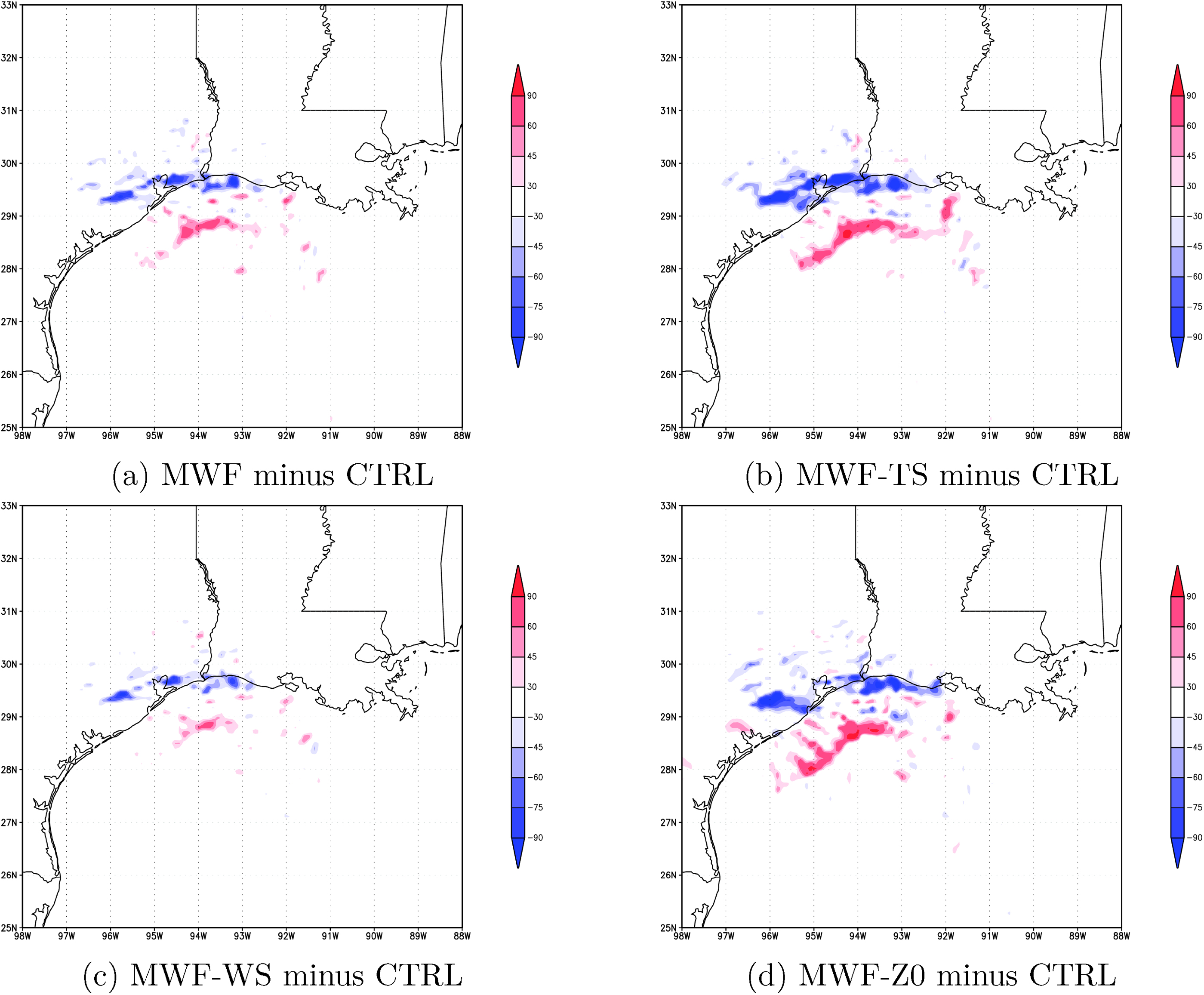
In addition to the wind farm cases modeled with the Fitch wind farm parameterization, case MWF-Z0 was run with a different treatment of the effect of the wind farms, namely, an increase in the value of surface roughness z0 only over the wind farm area. Although overly simplified, as wind farms are elevated, not surface-based, drag elements (Fitch et al 2013, Jacobson and Archer 2012), increasing surface roughness is a treatment of wind farms used in many studies in the past (Keith et al 2004, Kirk Davidoff and Keith 2008, Barrie and Kirk Davidoff 2010, Wang and Prinn 2010, Miller et al 2011). There is not a well-established method to determine by how much surface roughness should be increased to better represent the effect of wind farms. In the literature, a series of values ranging from 0.12 m to 3.4 m values have been proposed (Calaf et al 2010, Wang and Prinn 2010, Jacobson and Archer 2012, Fitch et al 2013). Here we tested several values between 0.2 m and 0.8 m and compared the resulting wind speed profiles averaged over the wind farm area to identify which gave a distribution of wind speed around hub height that was closest to that of the MWF case. The selected value of surface roughness is 0.5 m and the case is named MWF-Z0.
Results from MWF-Z0 confirm that precipitation is reduced inland and increased offshore, with a spatial pattern overall similar to that of the previous cases (figure 7(d)), although closest to the results from the case with tight inter-turbine spacing (MWF-TS in figure 7(b)) in terms of magnitude. This suggests that using an increased value of surface roughness may exaggerate the effects on precipitation overall, although the spatial distribution of the precipitation change was such that the Houston area was less affected with MWF-Z0 and SWF than with the other cases. At the same time, the comparison against the MWF-Z0 results was useful because it confirmed that offshore wind farms can impact the precipitation distribution during a hurricane such as Harvey regardless of the details of the wind farm parameterization used. Note that the idea of treating offshore wind farms as increased surface roughness is consistent with treating them as an 'extension' of the land into the ocean. Previous studies (Ogino et al 2016, Ogino et al 2017) have found precipitation maxima along the coast during tropical storms, where convergence occurs due to the slowing down of the winds, consistent with the precipitation enhancement found here upstream of the offshore wind farms.
To highlight the sensitivity of the precipitation to different layouts and parameterizations, table 3 shows a summary of the precipitation reduction of all the cases in the sector covering south Houston, described previously in section 3.1. The LWF and MWF simulations achieve almost the same benefit (∼15%), despite the fact that the LWF simulation includes more than twice the number of turbine of MWF. Increasing the number of turbines in the same area as MWF causes a larger reduction in precipitation (MWF-TS: 21.17%) and, vice versa, decreasing the number of turbines causes a smaller reduction (MWF-WS: 12.08%). Although the MWF-Z0 case shows a stronger precipitation reduction than MWF inland (figure 7), the percentage of precipitation reduction in the Houston area is lower than that of MWF (10.41% vs. 15.29%). The SWF case has the lowest precipitation reduction in all the cases (9.54%), which is possibly due to the absence of turbines in the Galveston Bay.
Table 3. Summary of the results for all the simulation cases.
| Case ID | No. of turbines | Installed capacity (TW) | 72 hour precipitation change in Houston (%) |
|---|---|---|---|
| CTRL | 0 | N/A | N/A |
| LWF | 74 619 | 0.56 | 15.37 |
| MWF | 33 363 | 0.25 | 15.29 |
| SWF | 28 197 | 0.21 | 9.54 |
| MWF-WS | 22 242 | 0.17 | 12.08 |
| MWF-TS | 59 312 | 0.44 | 21.17 |
| MWF-Z0 | N/A | N/A | 10.41 |
4. Conclusions
The potential impacts of large arrays of offshore wind farms on precipitation during a hurricane are evaluated through the case study of Harvey (2017) employing the WRF model. The simulations are set up without data assimilation and vortex initialization to isolate the potential effects induced by the wind farms, which would not be represented in the observations. The simulation without wind farms (control case) generally captures the life cycle of Harvey, but the maximum wind speed and precipitation are underestimated, while the minimum sea level pressure is overestimated, in comparison with the observations. Overall, the simulation is considered to be adequate for the aims of this study.
A large array of offshore wind farms can have significant impacts on precipitation during a hurricane. This claim is proven through a series of simulation cases, with different layout configurations, inter-turbine spacings, and wind farm parameterizations. Precipitation is found to be reduced inland and increased offshore in all the wind farm simulations. However, the amount of precipitation reduction varies in the different cases. The location of the wind farm also matters. The wind farm makes a big difference only when the upstream wind is blowing from offshore to the land (upper-right side of the hurricane center in the Northern Hemisphere and for the Texas coast). The turbines on the other side of the hurricane center (i.e. lower-left) have a much weaker impact on precipitation. When the turbines are moved away from the coast, to respect a no-construction strip from the coast, the area with a significant reduction in precipitation also moves slightly offshore.
The alteration of precipitation patterns is caused by changes in horizontal wind divergence and in vertical velocity. Due to the reduced speed over the wind farm area, patterns of convergence upstream (offshore) and divergence downstream (inland) of the wind farms are formed, with consequent enhanced vertical motion upstream and reduced vertical motion downstream. As the turbines inhibit vertical upward movement of warm air downstream of the offshore wind farms (i.e. along the coast and even further inland), convection is partially offset and precipitation is therefore reduced. Vice versa, offshore and upstream of the wind farms, precipitation is enhanced. Although this study is focused on Hurricane Harvey, the mechanism proposed is expected to hold for any hurricane, although the exact impact on precipitation may vary with other hurricanes and coastlines.
Three different wind farm layouts, along with two inter-turbine spacings, are tested in this study. Even the case with the widest spacing and therefore the lowest number of turbines (22 242) is still a futuristic scenario, considering that the largest offshore wind farm today (Anholt) includes 111 wind turbines. The next phase of this study will identify the smallest array size that still has significant benefits, focusing on the optimal layout that would maximize this benefit while, at the same time, minimizing the turbine installation costs.
An important limitation of this study is that, with the current Fitch wind farm parameterization, no sub-grid scale effects are considered. All the wind turbines within a grid cell are treated the same way, without considering their positions within the layout or the wind direction effects. As the number of wind turbines in the same grid cell ranges from 16–64, there can be significant wake effects and power losses within the grid cell for certain wind directions, which are neglected in the current study. A new hybrid wind farm parameterization, which considers the wind turbine positions within the grid cell and is sensitive to wind direction (Pan and Archer 2018), will be applied in an upcoming study on the optimal layout and size of offshore wind farms to reduce flooding and precipitation during hurricanes.
As this is the first study to assess the potential effects of large offshore wind farms on precipitation during a hurricane, it is important to mention that other impacts, not necessarily all beneficial, may occur. For example, the possible reduction of inland precipitation not only during hurricanes but also during normal weather conditions needs be evaluated for the human, geo-physical, agricultural, and ecological systems, especially for locations that may be experiencing water scarcity. The impacts of large offshore wind farms are expected not to be limited to inland regions, but to include, for example, the ocean between the coast and offshore wind farms. There, the patterns of reduced wind speeds and horizontal divergence reported in this study for the atmosphere may have an impact on the mixing processes in the ocean system, including a potential exacerbation of aquatic hypoxia in the surface layer. Lastly, since the extraction of wind energy by wind turbines can be controlled to a certain extent by changing their yaw and/or pitch angles, it is possible to perform intentional weather modification with offshore wind turbines when certain unfavorable conditions are forecasted, although this may increase the liability of wind farm operators in the case of forecast errors.
Acknowledgments
This research was funded in part by the Magers Family Fellowship. The simulations were conducted on the Mills and Farber high-performance computer clusters of the University of Delaware.