

Abstract
The future response of the atmospheric circulation to increased anthropogenic forcing is uncertain, in particular due to competing influences of the large projected warming at the surface in the Arctic, and at upper-levels in the tropics. In the present study two ensembles of fully-coupled 21st century climate simulations are used to analyze changes in the wintertime eddy-driven jet in the North Atlantic and the relation to the well-defined thermal signatures of climate change. The models project a robust reinforcement of the eddy-driven jet and a decrease in waviness and blockings, that we attribute to a narrowing of the westerly flow in mid-latitudes. Composite analyses suggest that this signal is driven by the opposite influence of Arctic and tropical warming on each flank of the jet. We find that a significant portion of the multi-model spread in the jet metrics can be explained by the ratio between these two signals. The tug-of-war between the two effects influences by how much wintertime cold extremes diminish at the end of the 21st century. Models with dominant tropical warming (i. e. narrower and stronger eddy-driven jet) exhibit less decrease in cold extremes with climate change, due to the maintenance of cooler conditions in the subpolar North Atlantic and subarctic seas compared to models with a predominance of Arctic warming.
Export citation and abstract BibTeX RIS

Original content from this work may be used under the terms of the Creative Commons Attribution 3.0 licence.
Any further distribution of this work must maintain attribution to the author(s) and the title of the work, journal citation and DOI.
1. Introduction
How climate change will impact the densely populated areas in mid-latitudes depends in large measure on the response in the large-scale atmospheric circulation to increasing anthropogenic radiative forcing. An increase in upper-level latitudinal temperature gradient, in particular associated with a strong upper-troposphere tropical warming (referred to as UTW hereafter), forces a poleward shift of the eddy-driven jet stream5 (Held 1993, Yin 2005, Butler et al 2010, Riviere 2011, Barnes and Polvani 2013, Harvey et al 2013). Near the surface, however, the latitudinal temperature gradient decreases due to polar amplification, i.e. faster warming of polar than lower-latitude areas. This effect, particularly pronounced in the Northern Hemisphere (NH) and referred to as Arctic amplification (AA), is due to a combination of feedback mechanisms, including sea ice loss (Holland and Bitz 2003, Screen and Simmonds 2010).
The accelerated rate of Arctic sea ice loss and AA in recent decades (Stroeve et al 2012) has motivated numerous research on its potential consequences on the mid-latitude climate (Cohen et al 2014, Vihma 2014, Walsh 2014). For example, Francis and Vavrus (2012) hypothesized that AA could lead to a weaker mid-latitude westerly flow, and thereby increased meanderings of the jet stream and extreme events, including cold outbreaks and snowfall in winter. If they exist, such signals are still small when compared with internal variability in observations (Wallace et al 2014, Barnes and Screen 2015). Numerous sea-ice loss numerical experiments have been performed with a variety of general circulation models (GCMs) and/or protocols. To date, no consistent response of regional temperature and extreme weather in mid-latitudes has emerged (Vihma 2014, Walsh 2014, McCusker et al 2016, Overland et al 2016), although some studies show a cooling of mid-latitude continents with reduced Arctic sea ice (Honda et al 2009, Petoukhov and Semenov 2010, Liu et al 2012, Kim et al 2014, Kug et al 2015). Indeed, the sea-ice-driven atmospheric response appears to be model-dependent and sensitive to the internal variability (Screen et al 2014), and it depends on the spatial pattern of the sea ice forcing (Peings and Magnusdottir 2014, Screen 2017), its amplitude (Magnusdottir et al 2004) and on the sea-surface temperature background (Smith et al 2017). Although the regional temperature response is inconsistent across the numerical studies, most agree on the response of the zonal-average circulation to a decline in Arctic sea ice, with weaker westerlies on the poleward flank of the eddy-driven jet and a southward shift of the jet/storm tracks. In particular, this response is robust in ocean-atmosphere coupled simulations with artificially-induced Arctic sea ice loss as projected at the end of the 21st century (Deser et al 2015, Blackport and Kushner 2017, Screen et al 2018).
Still, AA is only one component of climate change. The large UTW signal projected by GCMs due to increased upper-level latent heat release in the tropics (Santer et al 2017), as well as weaker and wider Hadley cells in winter (Seo et al 2014), may counterbalance its effect on the mid-latitude atmospheric circulation (Deser et al 2015, Blackport and Kushner 2017, Oudar et al 2017, McCusker et al 2017, Zappa and Shepherd 2017, 2018). In fact, in the zonal average, 21st century climate projections from the Coupled Model Intercomparison Project phase 5 (CMIP5) and from the Community Earth System Model Large Ensemble (CESM-LENS) show unchanged or slightly decreased mid-latitude waviness and frequency of blocking events, as well as reinforced westerlies at the core of the jet (Barnes and Polvani 2015, Cattiaux et al 2016, Peings et al 2017). This is opposite to expectations from the influence of AA alone (Francis and Vavrus 2012, Zappa et al 2018). Nevertheless, changes are highly sector-dependent (Peings et al 2017), the North American sector being the sole region to exhibit AA-expected changes (i.e. weakened westerly flow and increased waviness) (Cattiaux et al 2016, Peings et al 2017, Vavrus et al 2016). Over the North Atlantic, and to a lesser degree the North Pacific region, CMIP5 and CESM-LENS project a stronger zonal flow and decreased waviness/blockings (Cattiaux et al 2016, Peings et al 2017). In Peings et al (2017), we have linked this North Atlantic response in CESM-LENS to a narrowing of the westerly flow, under opposite influence of Arctic and tropical warming on each side of the jet. However, since CESM-LENS only accounts for uncertainties due to internal variability, it exhibits a small spread in AA and UTW. This hampers a robust evaluation of their respective contribution to future changes in mid-latitude dynamics, motivating further analyses with a multi-model ensemble that also includes model uncertainties.
In the present study we explore the changes in the North Atlantic atmospheric circulation by using 36 CMIP5 models and CESM-LENS, which allow us to quantify both model uncertainty and internal variability. We focus on the North Atlantic only, since all sectors cannot be investigated in details in one single study. The North Atlantic is of particular interest because it is, with the North Pacific, a region of maximum eddy-driven jet and baroclinic activity in winter, that impact the climate of Europe and eastern North America. The atmospheric response in the two ensemble of simulations is described using various dynamical metrics that capture different characteristics of the zonal flow. The tug-of-war between the effect of Arctic versus tropical changes is then discussed, as well as its impact on the projected response of cold extreme temperature over Europe.
2. Methods
2.1. Model data
We use an ensemble of 36 historical and RCP8.5 simulations from CMIP5, over the 1961–2095 period. The list of models included is given in table S1 available at stacks.iop.org/ERL/13/074016/mmedia (we use one realization per model). Details on the CMIP5 protocol can be found in Taylor et al (2012). All model output is interpolated to a horizontal 1.9 × 2.5° grid and 17 vertical levels. We also use 40 ensemble members from the Community Earth System Model Large Ensemble (CESM-LENS, Kay et al 2015). Each ensemble member consists of a different realization of a coupled ocean-atmosphere 1920–2100 simulation, forced by historical then RCP8.5 radiative forcing. The ensemble members only differ by perturbations in atmospheric initial conditions, giving an estimate of the importance of internal variability in the climate change response.
2.2. Description of the dynamical metrics
A variety of metrics are used to characterize the mid-latitude atmospheric dynamics in the model outputs. They are defined as follows:
- The zonal index (ZON) measures the strength of the average zonal flow in a given longitudinal sector. It is defined as the difference between 500 hPa geopotential height (Z500) in the high-latitudes (60–90°N) and in the mid-latitudes (20°–50°N).
- The sinuosity metric (SIN) is similar to the one described in Cattiaux et al (2016). For every day, the average Z500 between 30°N and 70°N is defined as the reference isohypse, the length of which is measured and divided by the length of the 50°N latitude circle. Sinuosity is therefore a ratio greater than 1 (1 representing a perfectly zonal flow), that measures the waviness of the mid-latitude (50°N) flow over a given longitudinal sector.
- Blocking events in mid-latitudes are identified using the 1-D blocking index (BLO) from Tibaldi and Molteni (1990), i.e. by identifying reversals in the Z500 meridional gradient that persist for at least 5 days.
- The jet width index (JWI) is derived from the average 30–70°N daily Z500 contours. For each month, the daily contours are zonally-averaged over the longitudinal sector, and a Gaussian fit is applied to the latitudinal distribution of the contours. The jet width is then defined as the latitudinal band that includes 95% of the daily contours (in ° latitude).
2.3. Climate change indices
Several large-scale signals of climate change are defined as follows:
- UTW is defined as the zonal mean temperature change in the (20°S/20°N; 400–150 hPa) domain.
- AA is defined as the zonal mean temperature change in the (60°N/90°N ; 1000–700 hPa) domain.
- The ratio UTW divided by AA is referred to as the RUTAW ('ratio between upper-troposphere tropical and Arctic warming') index.
- The polar stratospheric temperature (PST) is defined as the zonal mean temperature in the (70°N/90°N; 250–30 hPa) domain.
- UPTG is the upper-troposphere temperature gradient, computed as the difference between the zonal temperature in (20°S/20°N; 400–150 hPa) and (70°N/90°N; 400–150 hPa). LOTG is the lower-troposphere temperature gradient, computed as the difference between the zonal-mean temperature in (20°S/20°N; 1000–700 hPa) and (70°N/90°N; 1000–700 hPa).
- The Hadley cell width (HCW) is defined following Stachnik and Schumacher (2011). HCW is the distance (in degree-latitude) between the first latitude where the 700–400 hPa average value of the meridional streamfunction equals zero in each hemisphere.
- SSTG45 is the average meridional gradient of SST in the (45°N/55°N; 80°W/30°W) domain.
- Change in cold extreme temperature is assessed defining cold days at each grid point, based on the 1976–2005 distribution of minimum daily temperature of each model. A day that has its minimum temperature below the 10th percentile (Q10) of the present-day distribution is defined as a cold day, and the deviation from Q10 as the cold day anomaly (always negative). Then we sum the cold day anomalies for each month to construct a cold day intensity (CDI) index, expressed in degree-day. This metric allows us to account for changes in both the frequency and intensity of cold days.
2.4. Statistical analyses
Late 21st century changes are expressed as the difference between 2066–2095 and 1976–2005 in CMIP5, 1981–2010 and 2071–2100 in CESM-LENS. All analyses are October–March (ONDJFM) seasonal averages. The statistical significance of the anomalies is assessed using a two-tailed Student t-test.
3. Results
3.1. Changes in the atmospheric circulation over the North Atlantic
Figure 1 depicts the future minus present-day changes in zonal wind, at 700 hPa (U700, figures 1(a) and (d)) in zonal average (figures 1(b) and (e)), and as a function of time for U700 (figures 1(c) and (f)), over the North Atlantic sector (40°W–50°E). In both CMIP5 and CESM-LENS, we identify a tripole of zonal wind anomalies in the lower troposphere, with decreased westerlies on both flanks of the jet, and increased westerlies at its core (figures 1(a), (b), (d) and (e)). This signal represents a narrowing of the eddy-driven jet, as previously discussed in Peings et al (2017) for CESM-LENS. It is only found in winter (that we define as the 'extended-winter' October–March season) and it is more pronounced in OND in CMIP5, and JFM in CESM-LENS (not shown). The good agreement across a large ensemble of models (CMIP5) and different realizations of a single model (CESM-LENS) proves that it is a robust feature of RCP8.5 projections (note that the statistical significance is generally higher for CESM-LENS than for CMIP5, due to larger variance in CMIP5 that includes model uncertainty). The narrowing of the eddy-driven jet emerges significantly around 2070, starting with decreased winds on the poleward flank of the jet followed by a reduction on the equatorward flank (figures 1(c) and (f)). The narrowing signal over the North Atlantic dominates the zonal average but it is very sector-dependent (figure S1). The North Pacific sector also exhibits a narrowing of the jet (figure S1), although with less amplitude, while the jet tends to shift southwards over North America (Vavrus et al 2016).
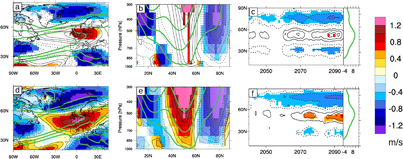
Figure 1. (a) CMIP5 ensemble mean of future vs present-day changes in 700 hPa zonal wind. (b) Cross-section of zonal wind changes averaged over the North Atlantic sector (50°W/40°E). (c) Latitude vs time change in 700 hPa zonal wind over the North Atlantic sector (50°W/40°E). (d), (e), (f) are the corresponding fields in CESM-LENS. Season is ONDJFM. Shading indicates anomalies that are significant at the 95% confidence level. Climatology is shown in green contours: 3 m s−1 interval on (a) and (d), 5 m s−1 interval on (b) and (e), sector zonal average in right panels of (c) and (f).
Download figure:
Standard image High-resolution imageIn order to further characterize the changes in the mid-latitude circulation, we use the ZON, SIN, BLO and JWI indices, that respectively measure the strength, waviness, reversal and width of the zonal westerly flow at 50°N over the North Atlantic. Their temporal evolution in CMIP5 and CESM-LENS is shown in figure 2, along with their future minus present-day mean change. On average, at the end of the 21st century, the zonal index shows a small increase in both ensembles of simulations (figure 2(a)), while sinuosity and blocking decrease by about 10% and 20%, respectively (figures 2(b) and (c)). This average response is opposite to the hypothesized effect of Arctic Amplification (i.e. increased waviness/blocking with weaker westerlies in mid-latitudes, Francis and Vavrus 2012), consistent with results from numerical sensitivity studies (Oudar et al 2017, McCusker et al 2017). The significant decrease in JWI (figure 2(d)) reflects the narrowing of the eddy-driven jet identified in figure 1. Our interpretation of these results is that a narrower (and stronger) jet allows for less meandering around its mean position, leading to less waviness and blocking events in the circulation (Barnes and Polvani 2013).
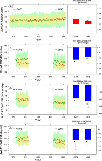
Figure 2. (a) Timeseries of the ONDJFM zonal index over the North Atlantic sector (50°W/40°E) in CMIP5 (green) and CESM-LENS (orange). Solid line is the ensemble mean, the envelope shows +/− 1 standard deviation spread between the models/members. The right panel shows the future versus present-day relative changes in %, with the +/− 1 standard deviation spread. A star indicates that the change is significant at the 90% confidence level. (b) Same as (a) but for sinuosity (relative future versus present-day changes are given, in %). (c) Same as (a) but for the blocking index. (d) Same as (a) but for the jet width index (future versus present-day changes are given in degree of latitude). ZON is computed from monthly data downloaded for the whole period. SIN, BLO and JWI are computed from daily data downloaded for two time slices.
Download figure:
Standard image High-resolution image3.2. Respective role of Arctic versus tropical changes in shaping the mid-latitude atmospheric response
The circulation changes described in the previous section exhibit a large spread, both among CMIP5 GCMs and CESM-LENS ensemble members (cf envelopes and error bars in figure 2). In this section we aim to understand which are the main drivers that cause this spread. In particular, models present a range of sensitivities in terms of future temperature changes. Figure 3(a) show the change in zonal mean temperature in CMIP5 (it is very similar in CESM-LENS). Apart from the well-known tropospheric warming/ stratospheric cooling response, two signals stand out in the temperature anomaly pattern: the strong UTW and the surface AA signal. As CMIP5 combines both model uncertainty and internal variability, it presents a larger spread than CESM-LENS (internal variability alone) in UTW and AA (figures 3(b) and (c)). CMIP5 is therefore more helpful than CESM-LENS to highlight the role of UTW and AA in shaping the response of the mid-latitude atmospheric circulation. However, CESM-LENS gives us an estimate of uncertainties due to internal variability, that we use in figure 4 to estimate the error that is made when using a single realization of a model.
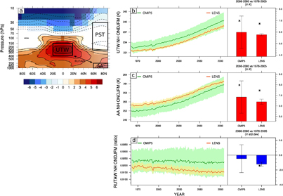
Figure 3. (a) CMIP5 ensemble mean of future vs present-day changes in ONDJFM zonal mean temperature. Shading indicates anomalies that are significant at the 95% confidence level. (b) Timeseries of ONDJFM UTW in CMIP5 (green) and CESM-LENS (orange). Solid line is the ensemble mean, the envelope shows +/− 1 standard deviation spread between the models/members. The right panel barplot shows the future versus present-day changes, with the +/− 1 standard deviation spread. A star indicates that the change is significant at the 90% confidence level. (c) Same as (b) but for AA. (d) Same as (b) but for RUTAW.
Download figure:
Standard image High-resolution imageTable 1. Matrix of correlations between the North Atlantic changes in the dynamical metrics (rows) and large-scale temperature/climate indices (columns) in the spread of CMIP5 models. BLO: blocking index—SIN: sinuosity index—ZON: zonal index—JWI: jet width index—TGLO: global mean surface temperature—AA: Arctic amplification—UTW: upper-troposphere tropical warming—PST: polar stratosphere temperature—RUTAW: ratio of UTW and AA—UPTG: upper-troposphere latitudinal temperature gradient—LOTG: lower-troposphere latitudinal temperature gradient—HCW: Hadley cell width—SSTG45: meridional gradient of SST at 45°N in the North Atlantic. Only correlations that are significant at the 95% confidence level are shown. For each dynamical index, the highest correlation is in bold, and the percentage of variance explained by the best 2-predictor linear regression model is given in the rightmost column.
| AT | TGLO | UPTG | LOTG | UTW | AA | PST | RUTAW | HCW (NH) | SSTG45 (AT) | Best 2 predictors model |
|---|---|---|---|---|---|---|---|---|---|---|
| BLO | −0.58 | −0.68 | −0.65 | −0.57 | — | 0.55 | UPTG+SSTG45 61% | |||
| SIN | −0.41 | −0.59 | −0.52 | 0.55 | −0.58 | −0.41 | 0.47 | PST+RUTAW 43% | ||
| ZON | 0.41 | 0.62 | −0.45 | 0.79 | — | — | PST+RUTAW 66% | |||
| JWI | −0.44 | −0.6 | −0.55 | 0.49 | −0.62 | — | 0.52 | RUTAW+SSTG45 50% |
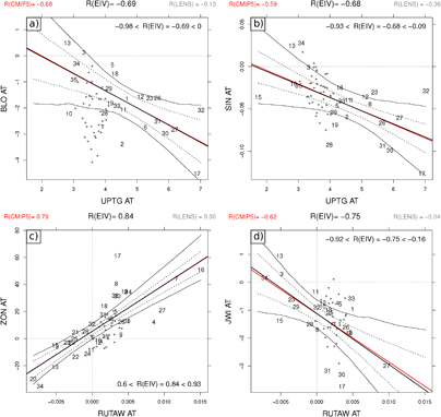
Figure 4. Scatterplots of ONDJFM future vs present-day changes in CMIP5 (numbers, see list in table S1) and CESM-LENS (grey dots) for: (a) BLO vs UPTG; (b) SIN vs UPTG; (c) ZON vs RUTAW; (d) JWI vs RUTAW. Results from three regression analyses are shown. The red solid lines and upper-left correlation coefficients (red) are for a standard regression analysis on CMIP5. The black solid lines and upper-center correlation coefficients (black) are for an error-in-variable regression analysis on CMIP5, using the CESM-LENS spread as errors on variables X and Y. The solid black curves gives a confidence interval for uncertainties due to both sampling error and internal variability. The dashed black curves are for uncertainties due to internal variability only (see appendix). The upper-right correlation is for a standard regression analysis on CESM-LENS.
Download figure:
Standard image High-resolution imageA large combination of inter-model regression analyses between the changes in dynamical indices (ZON, SIN, BLO and JWI) and in climate change indices listed in section 2.3 have been computed. In addition to UTW and AA, we compute regressions using the global mean surface temperature (TGLO), the upper- and lower-troposphere latitudinal temperature gradients (UPTG and LOTG, respectively) and the PST (their respective timeseries/mean changes are shown in figure S2). The spread in TGLO (figures S2(a)) represents the diversity in climate sensitivity among the models (it is, as expected, very small in CESM-LENS). UPTG increases in the model due to UTW, while LOTG decreases with AA (figures S2(b) and (c)). Future changes in PST are more model-dependent and internally-driven than UTW and AA (cf large spread in figure S2(d)), as expected from high internal variability in the stratosphere (Manzini et al 2014). Since UTW and AA are both correlated with TGLO, it is difficult to isolate their respective influence on the dynamical changes. For this reason, we use the RUTAW index, simply defined as the ratio between UTW and AA6. Unlike UTW and AA, RUTAW does not exhibit a significant trend over the 21st century in CMIP5, with a large spread between the models (figure 3(d)). Therefore, RUTAW allows us to efficiently separate the models that have a strong UTW relative to AA (positive RUTAW), from the models that exhibit a dominant AA versus UTW (negative RUTAW) (see figure S3). We also include an index of Hadley cell expansion (Hadley Cell Width, HCW), in order to assess whether this robust climate change signal in both CMIP5 and CESM-LENS (figures S4(a) and (b)) is a driver of the mid-latitude dynamical changes. A last index is the meridional gradient of sea surface temperature (SST) at 45°N in the North Atlantic (SSTG45, figures S4(c) and (d)), SST gradients in the Gulf Stream region being a potential driver of baroclinicity hence of the downstream atmospheric flow (O'Reilly et al 2017).
Correlation coefficients of the standard regression analyses are summarized in table 1, along with the variance explained by the best 2 predictor linear regression model used to predict each dynamical index. Note that all the indices but HCW are zonally-averaged over the North Atlantic sector (similar results using the NH zonally-averaged indices are given in table S2). The scatterplots corresponding to the highest correlation found for each dynamical index are shown in figure 4, using an error-in-variable (EIV) regression that uses the CESM-LENS spread to estimate uncertainties due to internal variability alone (see appendix for description of the method). The highest correlation is found between RUTAW and ZON (REIV = 0.84 with a 95% confidence interval of 0.59/0.93, figure 4(c)). RUTAW explains significantly more variance in ZON than UTW and AA alone (table 1). The positive correlation indicates that GCMs with greater warming in the tropics relative to the Arctic have positive ZON anomalies over the North Atlantic (i.e. positive North Atlantic Oscillation), and conversely. When coupled with PST, the multiple regression model RUTAW+PST explains 66% of the variance in ZON. RUTAW also exhibits the highest correlation with JWI (figure 4(d)), while BLO and SIN are more strongly correlated with UPTG (figure 4(a)–(b)). SSTG45 also emerges as a good predictor of BLO, SIN and JWI (table 1), although a causal relationship is difficult to assess because of the two-way relationship between atmospheric and SST changes. HCW is negatively correlated with SIN, i.e. models with a stronger HC expansion tend to be the ones with less waviness in the mid-latitude flow. Corresponding correlations using the CESM-LENS spread (grey dots in figure 4, and table S3) are smaller, especially with RUTAW, UTW and AA, as expected due to the absence of model uncertainty.
Overall, these results suggest that the competition between AA and UTW (represented by RUTAW) can explain a significant part of the multi-model spread in changes of the zonal westerly flow over the North Atlantic (ZON and JWI). In general, GCMs with dominant tropical warming project a stronger and narrower westerly flow, while GCMs with larger Arctic warming respond the opposite way. Synoptic metrics (BLO and SIN) appear to be more sensitive to changes in the upper-troposphere temperature gradient, with less influence of Arctic Amplification. Consistent with previous studies (Manzini et al 2014, Zappa and Shepherd 2017, Peings et al 2017), we also find a connection with the polar stratospheric temperature. SIN and JWI decrease more strongly in models/members with a cooler polar stratosphere (PST) at the end of the 21st century. Whether the stratosphere drives or responds to the tropospheric changes is not addressed in this study, but this is a robust link both in CMIP5 (table 1) and CESM-LENS (table S3).
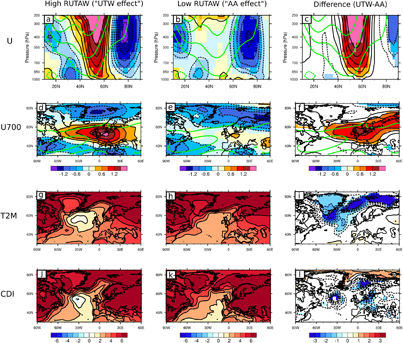
Figure 5. (a) Composite of ONDJFM change in winter zonal wind over the North Atlantic sector for CMIP5 models with a high RUTAW ('UTW effect'). Shading indicate anomalies that are significant at the 95% confidence level. Climatology is in green contours (5 m s−1 interval). (b) Same as (a) but for CMIP5 models with a low RUTAW ('AA effect'). (c) Difference between (a) and (b), i.e. high minus low RUTAW models. (d)–(f) Same as (a)–(c) but for zonal wind at 700 hPa (climatology: 6 m s−1 interval). (g)–(i) Same as (d)–(f) but for 2 meter temperature. (j)–(l) Same as (d)–(f) but for cold days intensity.
Download figure:
Standard image High-resolution image
In order to further highlight the respective influence of UTW and AA on the mid-latitude atmospheric response, we composite the CMIP5 models based on their future vs present-day change in RUTAW index. The six models with the highest change in RUTAW ('UTW effect') are compared to the six models with the lowest change in RUTAW ('AA effect'). The corresponding zonal temperature anomalies over the North Atlantic are shown in figures S3(a). Note that such an analysis using CESM-LENS is not effective, due to the lack of variability in RUTAW to efficiently separate UTW from AA (figures S3(b)). The UTW-effect models project a reinforcement and slight poleward shift of the eddy-driven jet (figures 5(a) and (d)), a signal that is absent in the AA-effect models, in which the main signal is a significant reduction in the westerlies on the poleward flank of the jet (figures 5(b) and (e)). Although reduced, AA is still present in the high-RUTAW composite, as is UTW in the low-RUTAW composite (figure S3(a)), but their difference maximize the signal and reveal their competing influences (figures 5(c) and (f)). In the absence of AA, the eddy-driven jet would migrate poleward over the eastern Atlantic and Europe, as expected from an increase in upper-level meridional temperature gradient (figure 5(f)). However, AA counteracts this effect by reducing the westerlies on the poleward flank of the jet, in agreement with Zappa et al (2018), and recent numerical sensitivity studies (Deser et al 2015, Blackport and Kushner 2017, Oudar et al 2017, McCusker et al 2017). The two effects combine in producing a narrowing and decreased waviness/blocking of the flow.
3.3. Implications for mean and extreme temperature changes over Europe
Figures 5(g)–(i) shows the changes in 2 meter temperature (T2M). Not surprisingly, the temperature strongly increases almost everywhere, especially over continental and high-latitude areas. However, models with a stronger UTW-effect exhibit less warming along the path of the reinforced jet, from the south of Greenland to the Barents Sea (figure 5(i)). This cooling is associated with cooler SST in the subpolar regions (figures S5(d)–(f)). Such signal may be partly driven by the jet reinforcement and increased wind stress and turbulent heat flux exchanges at the surface. However, oceanic processes also play a role. In particular, a weaker Atlantic meridional overturning circulation (AMOC), a response projected by CMIP5 models at the end of the 21st century and beyond (Cheng et al 2013), is associated with decreased deep convection and cooler SST in the subpolar North Atlantic (Sgubin et al 2017). In particular, cold SST anomalies in the subpolar gyre (or 'North Atlantic warming hole', Drijfhout et al 2012) is a marker of a weaker AMOC, and we find it is more pronounced in UTW-effect models (figures S5(d)–(f)). Moreover, the UTW-effect models show less decrease in Arctic sea ice (figures S5(c)) and warmer SST in the South Atlantic (figures S5(f)), two signals that are consistent with a reduced AMOC and decreased heat transport in high-latitudes. A decreased meridional heat transport is also consistent with a warmer tropical atmosphere, i.e. a higher RUTAW, since more energy accumulates in the tropics. The significant correlation between the intensity of the North Atlantic warming hole and RUTAW (figure S6) supports this interpretation, although further analyzes of oceanic variables will be needed to explore this question in more detail. The role of the AMOC and ocean dynamics in the Arctic-versus-tropics tug-of-war is an interesting prospect for future studies.
Finally, we show how the different jet responses affect extreme temperature over Europe. From a dynamical perspective, with a stronger westerly flow, one might expect even less cold extremes in winter in the dominant UTW-effect models, due to reduced north-south excursions of the jet and associated cold air outbreaks. Actually, the intensity of cold days (CDI, see definition in section 2.3) decreases less in the UTW-effect models than in the AA-effect ones, especially over Western Europe (figures 5(j)–(l), Łpositive values represents a decrease in CDI). This can be explained by thermodynamical changes in high-latitudes, that counteract changes in dynamics (Ayarzagüena and Screen 2016). Although a stronger westerly flow allows for less meandering of the jet, the reduced surface warming in high-latitudes, promoted by cooler SST in the subpolar Atlantic (figures S5(f)) and less sea ice loss in the Barents-Kara sea (figures S5(c)), results in cooler air advection from the north-east during cold air outbreaks than in models with a dominant AA-effect. Again, it will be interesting to quantify the respective role of atmosphere and ocean dynamics processes (i.e. AMOC) in dedicated sensitivity GCM experiments.
4. Conclusion
Our analyses of RCP8.5 scenarios highlight the competition of Arctic versus tropical warming in the response of the North Atlantic eddy-driven jet. We argue that the response of the jet does not consist of a latitudinal migration that could be expected from changes in upper- or lower-level temperature gradients alone, but from their combination that results in a narrowing and reinforcement/elongation of the westerly flow. This interpretation helps to reconcile the discrepancy between the hypothesized impact of Arctic amplification (Francis and Vavrus 2012, Cohen et al 2014) and the actual changes in mid-latitude dynamics (less sinuosity, less blocking) in the RCP8.5 projections of the late 21st century (Barnes and Polvani 2015, Cattiaux et al 2016, Peings et al 2017). The spread among the models is large, but we show that better agreement is found when using RUTAW to differentiate the models.
In observations/reanalyses, a small but statistically significant trend towards increased sinuosity has been detected over the North Atlantic sector (Francis and Vavrus 2012, Cattiaux et al 2016). It is consistent with the large AA observed over the recent period, while, to date, UTW has remained modest compared to model projections (Santer et al 2017). Our results suggest that we can expect this trend to reverse in future, once UTW emerges strongly in observations with unabated anthropogenic emissions, reduction of the AMOC, and associated warming of tropical SST.
Appendix
Standard linear regressions and correlations in figure 4 are obtained from CMIP5 single-run points (X,Y) in a ordinary least squares (OLS) framework. An error-in-variable framework is also used to estimate the slope on the true CMIP5 points (X⁎,Y⁎), i.e. the slope which would be obtained if we had numerous realizations for every CMIP5 model and computed the OLS regression on ensemble mean points. The mathematical framework to derive the error-in-variable slope and associated correlation is described here.
Let (X,Y) be the random variables of single-run CMIP5 values, and (X⁎,Y⁎) the random variables of true CMIP5 values. Both are linked with an error term resulting from internal variability:

The linear regression model on (X⁎,Y⁎) writes:

with an estimator of the slope beta given by:

Similarly, the slope of the regression model on (X,Y) is estimated by:

Under the reasonable assumption that errors in X and Y are uncorrelated from X and Y, the covariance matrix of (X,Y) can be decomposed as:
This leads to:

with:
The error-in-variable estimate of the slope (beta hat) is therefore a correction of the standard estimate (beta tilde) accounting for the errors in X and Y, and knowing the covariance matrix of the errors. Here we estimate this covariance matrix from CESM-LENS, assuming that all CMIP5 models have a similar internal variability.
We compute the correlation coefficients (r) as the root mean square of the fraction of variance in Y that is explained by the regression of X. We derive two r coefficients corresponding to the two betas:

Finally, confidence intervals on the regression lines are obtained from a bootstrap procedure that accounts for both sampling error and internal variability. For each pair of variables (X,Y), 10000 iterations are made. At each iteration, the CMIP5 couples (Xi,Yi) (i in 1..N) are perturbed by a vector (xj,yj) (j in 1.. n), randomly drawn among deviations of CESM-LENS individual realizations from their ensemble mean. This is meant to represent how internal variability has affected the CMIP5 point cloud. Then a random selection of N couples (Xi-xj,Yi-yj) is made among the N couples (with replacement) as classically done in regression analysis to account for sampling error. Both OLS and EIV estimates of the slope are computed, and once the 10000 iterations are done, the quantiles 0.025 and 0.975 provide the 95%-level confidence intervals that are shown (solid lines). Repeating the same procedure without the second step (resampling) provides the 95%-level confidence interval representing internal variability only (dashed lines).
Acknowledgments
We thank the editor and two anonymous reviewers for their help in improving this study. Thanks are due to Clara Deser, Adam Phillips, the CESM Large Ensemble Community Project and supercomputing resources provided by NSF/CISL/Yellowstone for making the CESM-LENS data available. We acknowledge the World Climate Research Program's Working Group on Coupled Modelling, which is responsible for CMIP, and we thank the climate modeling groups for producing and making available their model output. YP and GM are supported by NSF Grant AGS-1624038.
Footnotes
- 5
Lower-troposphere westerly winds of mid-latitudes that both drive and result from the storm tracks through eddy-mean flow interactions.
- 6
Another method to isolate the role of UTW and AA would be to divide them by the global mean temperature (Zappa and Shepherd 2017), but our approach presents the advantage of using a single index since the ratio cancels the influence of TGLO.