

Abstract
The assessment of regional climate change and the associated planning of adaptation and response strategies are often based on complex model chains. Typically these employ global and regional climate models (GCMs and RCMs), as well as one or several impact models. It is a common belief that the errors in such model chains behave approximately additive, thus the uncertainty should increase with each modeling step. If this hypothesis was true, the application of RCMs would not lead to any intrinsic improvement (beyond higher-resolution details) of the GCM results. Here, we investigate the bias patterns (offset during the historical period against observations) and climate change signals of two RCMs that have downscaled a comprehensive set of GCMs following the EURO-CORDEX framework. Our results show that the biases of the RCMs and GCMs are not additive and not independent. The two RCMs are systematically reducing the biases and modifying climate change signals of the driving GCMs, even on scales that are considered well resolved by the driving GCMs. The GCM projected summer warming at the end of the century is substantially reduced by both RCMs. These results are important, as the projected summer warming and its likely impact on the water cycle are among the most serious concerns regarding European climate change.
Export citation and abstract BibTeX RIS

Original content from this work may be used under the terms of the Creative Commons Attribution 3.0 licence.
Any further distribution of this work must maintain attribution to the author(s) and the title of the work, journal citation and DOI.
1. Introduction
While climate change is a fundamentally global problem, driven by anthropogenic changes in atmospheric constituents and land-use, the impacts of climate change inevitably require consideration of regional effects (IPCC 2014). In particular, the simulation of meso-scale atmospheric structures, such as precipitating weather systems and fronts, is improved by higher model resolution. In addition, the development of adaptation and response strategies rely strongly on regional information and often depends on smaller-scale geographical features, such as coastlines and mountain areas. On an institutional level, the need for regional climate change information is reflected in the formation of climate services, which have a strongly national and regional orientation (Fischer et al 2012a, Goddard 2016, Kjellström et al 2016, Adams et al 2015). The importance of an adequate assessment of the associated uncertainties has been emphasized in a number of studies (Déqué et al 2012, Hawkins and Sutton 2009).
To gain high-resolution regional climate information for this purpose, regional climate models (RCMs) are used as a dynamical downscaling tool. The methodology involves driving an RCM at its lateral boundaries and most often the sea surface, using information from a lower-resolution global climate model (GCM) (Di Luca et al 2016, Giorgi and Mearns 1999, Rajczak et al 2013, Rajczak and Schär 2017, Rummukainen 2016). The approach was originally developed in the context of short and medium-range numerical weather prediction. Today, large ensembles of global and regional climate simulations are available through internationally coordinated projects such as CMIP5 (Taylor et al 2012) and CORDEX (Giorgi et al 2009). The available GCM and RCM simulations have horizontal grid spacings of typically 100–300 km and 10–50 km, respectively.
It is widely accepted that RCMs improve the representation of smaller-scale features compared to the driving GCMs, especially regarding the representation of precipitation in mountainous regions (Ban et al 2015, Frei et al 2003). It has also been shown that the added value over complex terrain is not only a result of better resolving the large-scale forcing fields, but that the technique yields an improved representation of the underlying physical processes (Torma et al 2015). Even in absence of topography, the higher resolution generates fine-scale structures within the RCM domain, with adequate amplitudes in the different climate components that are consistent with the observed climatological means (Di Luca et al 2016, Di Luca et al 2012, Di Luca et al 2015, Diaconescu and Laprise 2013, Torma et al 2015).
Nevertheless, in spite of this added value of RCMs compared to GCMs (Rummukainen 2016), there are two major concerns. The first one has been addressed with the paradigm of the 'cascade of uncertainty' (Mitchell and Hulme 1999). It describes how the uncertainties in a model chain are expanding from one step to another. More specifically, it is argued that 'the range (or envelope) of uncertainty expands in each step (of the model chain) to the extent that potential impacts and their implied adaptation responses span such a wide range as to be practically unhelpful' (Wilby and Dessai 2010). This 'cascade of uncertainty' assumes that the errors from the different steps of a model chain are essentially independent and additive.
Second, it is evident that RCMs cannot modify the larger-scale atmospheric circulation, and it is thus not obvious whether they can improve the larger-scale climate properties, such as the continental to sub-continental surface temperature distribution. This concern has been discussed in a number of influential papers and comments (Hall 2014, Kerr 2011, Kerr 2013, Schiermeier 2010). While GCMs undoubtedly produce useful results on the global scale, they have considerable biases on the scales used to drive an RCM. Using GCMs to drive RCMs is thus not necessarily producing more reliable results, but might merely yield 'more detailed noise' (Kerr 2013). This 'garbage in, garbage out' argument is frequently used in the discussions about how reliable a RCM is (Giorgi and Mearns 1999, Hall 2014, Kerr 2011, Kerr 2013, Rummukainen 2010, Schiermeier 2010).
Both the 'garbage in, garbage out' and 'cascade of uncertainty' statements are not giving an optimistic view of the regional climate modeling approach. Here we test these statements and show that the RCMs are systematically improving the GCM results. We use results from two regional models that have downscaled several GCMs over Europe, following the EURO-CORDEX framework (Giorgi et al 2009, Jacob et al 2014, Kotlarski et al 2014). Consideration will be given to summer 2 m air temperatures for current and future climate conditions under the RCP8.5 emissions scenario (Moss et al 2010). For this scenario, a large number of simulations are available from the EURO-CORDEX archive. At the time of writing, a total of ten different CMIP5 GCMs and 10 RCMs have been used in such simulations. However, from the possible GCM-RCM matrix of 10 × 10 simulations, only a fraction of combinations (27%) have been simulated (see www.euro-cordex.net for more information about the EURO-CORDEX and the full simulation list). Also, many of the CMIP5 GCMs have been run for a large number of realizations. Of these only a very small fraction has been downscaled by RCMs. Regrettably, a significant number of RCMs have only downscaled one or very few GCMs. Such simulations cannot be used in the current study, as there is no way to tell whether an improvement due to the RCM is by coincidence (e.g. due to compensation of errors) or intrinsic to the methodology. We are thus restricting the analysis to those RCMs that have downscaled at least five GCMs. In addition, we are only considering simulations with grid spacing of 50 km (but consideration of the simulations at 12.5 km resolution yields similar results).
These selection criteria pinpoint two RCMs, namely the Rossby Centre regional climate model (RCA Strandberg et al 2014) and the Consortium for Small-Scale Modelling in Climate Mode (COSMO Climate Limited-area Modelling, hereafter CCLM, Rockel et al 2008). The RCA has downscaled nine different GCMs, while CCLM has downscaled five GCMs. The simulation matrix of the different GCMs that have been downscaled by the two RCMs is given in table 1, and further details of the data and methodology are provided in section 2. The results are presented in section 3. We end with a discussion of the main findings in section 4, and conclusions in section 5.
Table 1. The simulation matrix. The column to the left lists the nine GCMs that have been dynamical downscaled by the two regional models CCLM and RCA4. For each model, the first line lists the model name and the country. The second line lists the horizontal grid spacing and the vertical resolution (if two numbers are listed for the horizontal resolution, these refer to longitude and latitude at the equator, respectively), and the last line provides the main reference. A cross is given when the GCM has been downscaled with the respective regional model, for the historical period (1950–2005) and with the RCP8.5 from 2006–2099. Both regional models have a horizontal resolution of 50 km and follow the Euro-CORDEX framework.
| GCM\RCM | CCLM (CLM-Com) | RCA4 (Sweden) |
|---|---|---|
| 50 km, 40 levels | 50 km, 40 levels | |
| Rockel et al (2008) | Strandberg et al (2014) | |
| CanESM2 (Canada) | ||
| 210 km (T63), 35 levels | X | |
| Arora et al (2011), Salzen et al (2013) | ||
| CNRM-CM5 (France) a | ||
| 160 km (TL127), 31 levels | X | X |
| Voldoire et al (2013) | ||
| EC-EARTH (Europe) | ||
| 80 km (T159), 62 levels | X | X |
| Hazeleger et al (2011) | ||
| GFDL-ESM2M (USA) | ||
| 280 × 220 km, 24 levels | X | |
| Dunne et al (2012), Dunne et al (2013) | ||
| HadGEM2-ES (UK) | ||
| 210 × 140 km, 38 levels | X | X |
| Collins et al (2011), Martin et al (2011) | ||
| IPSL-CM5A-MR (France) | ||
| 280 × 140 km, 39 levels | X | |
| Dufresne et al (2013) | ||
| MIROC5 (Japan) | ||
| 160 km (T85), 40 levels | X | X |
| Watanabe et al (2011) | ||
| MPI-ESM-LR (Germany) | ||
| 210 km (T63), 47 levels | X | X |
| Stevens et al (2013) | ||
| NorESM1 M (Norway) | ||
| 270 × 210 km, 26 levels | X | |
| Iversen et al (2013) |
aThe lateral boundary conditions from the GCM CNRM-CM5 is subject to some erroneous files. See supplementary information available at stacks.iop.org/ERL/13/074017/mmedia for more information.
2. Data and methods
We analyze nine different GCMs from the CMIP5 ensemble (listed in table 1 with their respective references) that have been used for dynamical downscaling by the two RCMs. The GCM model outputs of daily near surface temperature and accumulated precipitation are compared with the output from the RCMs. For analysis, the GCMs results have been interpolated to the EURO-CORDEX grid with 50 km horizontal resolution by using a conservative interpolation method.
The two RCMs we have used in this study were developed at different institutes in Europe i.e. RCA at SMHI (Strandberg et al 2014) and CCLM by the COSMO (COSMO 2018) and the CLM-community (CLM-COM 2018). The CCLM has downscaled five of the nine GCMs listed in table 1. CCLM is a non-hydrostatic model based on the numerical weather prediction model COSMO (Baldauf et al 2011, COSMO 2018), which has been developed into a regional climate model by the CLM-community (CLM-COM 2018) and is referred to as the CCLM (CLM-COM 2018, Rockel et al 2008). The number of vertical levels is 40 and the horizontal resolution is 0.44°, which corresponds to a 50 km grid spacing. In comparison to recent applications (Keuler et al 2016, Kotlarski et al 2014), the updated model version 5.0_clm6 is used, which is the latest recommended model version from the CLM-community. This model version has been comprehensively tested and has undergone an objective calibration (Bellprat et al 2016). The newer model version has been shown to reduce the CCLM model biases compared to older model versions, especially regarding reducing the warm (dry) summer temperatures (precipitation) biases over southern/southeastern Europe.
To distinguish the role of the different parametrization schemes from the resolution effect, we also performed an extra set of sensitivity experiments, where we decreased the horizontal resolution in CCLM to approximately 200 km. The coarse resolution sensitivity simulation with CCLM is using the exact same configuration as the 50 km simulations, except that the horizontal resolution is 1.760° (~200 km) and the domain has been increased by approximately 10° on each side, resulting in 43 × 42 grid points in total. In addition, the time step has been decreased to 1200s. The goal of this sensitivity experiment was to separate the parametrization effect from the resolution effect, but it should be noted that the set-up of parameterizations has not been optimized for this coarser resolution. The two GCMs that were downscaled were simulated from 1966–2000, where the five first years were removed due to spin-up.
The RCA simulations are performed by the swedish meteorological and hydrological institute (SMHI) and are available at https://esg-dn1.nsc.liu.se/projects/esgf-liu/. The RCA model has downscaled all the nine GCMs listed in table 1. The model version RCA4 is used at 0.44° (50 km) horizontal resolution, with 40 vertical levels. Details about the simulations can be found in Kjellström et al (2016) and Strandberg et al (2014).
Both the CCLM and RCA use the experimental setup following the EURO-CORDEX framework (EURO-CORDEX 2017, Jacob et al 2014, Kotlarski et al 2014). The RCMs are downscaling the respective GCMs for the historical period (1950–2005) and future projection based on the RCP8.5 scenario (2006–2100). With this approach, the flow of information is exclusively from the lower to the higher-resolution, i.e. from the GCM to the RCM (one-way nesting).
We are comparing the results from the RCMs with those of the corresponding driving GCMs. The time period 1971–2000 is used as reference, and the climate change signal is evaluated for the end of the century (2070–2099) relative to the reference period. The daily mean temperature (°C) and daily-accumulated precipitation (mm day−1) is calculated for each season (winter: December–January–February (DJF); spring: March–April–May (MAM); summer: June–July–August (JJA); fall: September–October–November (SON)). A height correction is applied to the GCM and RCM temperature fields to account for topographic differences between model and observations assuming a constant lapse rate of 0.65 K/100 m. This commonly used correction is important when considering biases, especially in the GCMs.
To calculate the temperature biases in the GCMs and RCMs, we are using version 13.1 of the daily gridded E-OBS dataset (Haylock et al 2008). E-OBS covers the whole of the European land surface, and combines observations from the European Climate Assessment and Dataset (ECA&D) with observations from many other databases over Europe. The Root mean square error (RMSE) is used to investigate the error in the different model ensembles. RMSE is defined as:
where Xn is the model result (GCM or RCM), and N is the number of simulations in the ensemble (N = 9 for the RCA ensemble, and N = 5 for the CCLM ensemble).
Furthermore, the RCM and GCM outputs are compared by aggregating the results over the eight PRUDENCE regions (Christensen and Christensen 2007) (see supplementary figure S1). Elements of our analyses follow previous studies, in particular regarding current-day model biases (Kerkhoff et al 2015) and of future climate changes (Kjellström et al 2016), but we provide a more thorough assessment of the climate change signal in terms of surface temperature and precipitation at the end of the century (2070–2099) relative to the historical period (1971–2000).
To visualize the climate change signal, a probability ellipse for the bivariate climate change signal is calculated, where the data are assumed to have a normal distribution. The covariance of the data determines the angle of the ellipse (Wilks 2011). The ellipse represents the contour of the confidence interval, which is set to one standard deviation, thus the probability ellipse covers 68.2% of the data. One caveat is that the probability ellipse is based on a small number of data points. For the CCLM ensemble only five data points are used to fit the probability ellipse for the bivariate climate change signal, whereas for the RCA ensemble nine data points are used. However, the probability ellipses are merely meant to guide the eye when considering the figure, rather than providing a probabilistic assessment.
3. Results
Figure 1 shows the root mean square error (RMSE) of the near-surface temperature from the raw GCM output (left-hand panels) and the same simulations but downscaled by the two RCMs (right-hand panels) for the summer season (June–July–August, JJA). The bias of each respective simulation is shown in figure S9. Top and bottom panels refer to the different samples of GCMs, namely the five GCMs that drive CCLM (top panels) and the nine GCMs that drive RCA (bottom panels). From figure 1 it is evident that the error is reduced from the GCMs to the RCMs in both samples. The large error in eastern Europe, seen in both the GCM ensembles, is strongly reduced in the two RCM ensembles. There are also some regions where the error is increasing with the RCMs. This is particularly seen over the Iberian Peninsula for the CCLM ensemble, and over the Alps and Scandinavia for the RCA-ensembles. In these regions, the respective RCMs have known model biases, which are seen when driving the RCM by ERA-Interim reanalysis lateral boundary conditions (Kotlarski et al 2012, Bellprat et al 2016, Strandberg et al 2014).
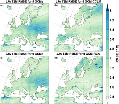
Figure 1. Root-mean-square-errors (RMSE) of summer near-surface temperatures, showing the reduction of the error from the GCMs to the GCM-RCM simulations. Left and right-hand panels show results for the raw GCMs, and the RCM simulations. Top and bottom panels are for the two ensembles using the CCLM (top) and RCA4 (bottom) regional climate models, respectively.
Download figure:
Standard image High-resolution imageTo better understand how the biases of the RCMs depend upon the driving GCMs, we perform a detailed analysis for four European regions (see figure S1 for the boundaries of the regions). More specifically, we display in figure 2 the RCM increment (defined as RCM–GCM) as a function of the GCM bias (defined as GCM–observations). If the RCM increments were independent of the GCM biases, then the distribution of data points should be uncorrelated. However, if the RCM increments systematically counteract the GCM biases, then the distribution will have a negative correlation, and if it enhances the bias there will be a positive correlation. If the RCMs were perfectly compensating the full GCM biases, then the data cloud would be aligned along the y = −x line. Comparing GCM biases with RCM increments in this fashion was first performed in Kerkhoff et al (2015), where temperature biases were studied in four European regions. They used data from the ENSEMBLES project (ENSEMBLES 2009) and showed that there is a negative relation between the GCM bias and the RCM increment, indicating that the RCMs compensate for some of the GCM biases. However, since at that time only few suitable simulations were available (several GCMs need to be downscaled by the same RCM), it was not evident whether the result was due to systematic behavior or merely coincidence.
The results in figure 2 are averages of the near surface temperature over Scandinavia, the Alps, the Iberian Peninsula and eastern Europe. In all four regions there is a negative relation between the GCM bias and the RCM increment, for both models (shown by different symbols). Even though the results are not perfectly aligned along the y = −x line, there is a clear systematic reduction of the GCM bias by the RCMs. In particular, it is evident that the RCM increments strongly depend upon the GCM and counteract the GCM biases. Consider for instance the effect over eastern Europe, where the GCM MIROC5 has a warm bias of almost 6 °C. This bias is counteracted by CCLM with an increment of −4 °C, thus the regional model is almost removing the bias in the model chain (figure 2(d), circle symbols). On the other hand, EC-EARTH has a small cold bias of about –0.8 °C, which is counteracted by CCLM with an increment of about 0.3 °C. The same effect is seen for the RCA model, where the RCA increment varies depending on the bias of the GCM. This shows that the RCM increment strongly depends upon the driving GCM, and there is a clear tendency that the RCMs are reducing the GCM biases. Over the Iberian Peninsula the relation between the GCM bias and RCM increment has its lowest performance, where both RCMs are having difficulties in correcting the cold GCM biases. As discussed in the context of figure 1, the CCLM has a significant model bias in this area (Bellprat et al 2016). Nevertheless, the negative correlations between the GCM bias and the RCM increment clearly show that the RCMs are systematically reducing the GCM biases.
The reduction of the bias is most evident during the summer season, when the large-scale flow and influence is less pronounced. In particular, for all regions considered (see supplementary figures S2–5 for additional regions and seasons), there is a negative correlation between the GCM bias and the RCM increments, i.e. the RCMs counteract the GCM bias in near-surface temperature. While the amplitude of the effect is weaker in the other seasons, the evidence is still strong. More specifically, for the 64 combinations tested (two RCMs, four seasons, eight regions), the correlations are negative in 63 cases. Hence the systematic reduction of the GCM bias by the RCMs cannot be by chance. There is a positive correlation only for the RCA model in spring over Scandinavia. This exception likely derives from some biases of the RCA related to the melt of the seasonal snow cover, which is simulated about one month later than observed (Strandberg et al 2014). It is also interesting that during winter, when the large-scale flow is more pronounced, the improvement by the regional models is still present, although somewhat weaker.
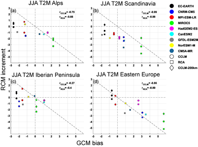
Figure 2. Systematic reduction of the GCM bias by the RCMs. The panels display the RCM increments (RCM–GCM) versus the GCM biases (GCM–OBS) for near-surface temperatures. Data points along the dashed diagonal signal an increased performance of the GCM-RCM simulations in comparison to the GCMs. The four panels relate to the Alps (a), Scandinavia (b), Iberian Peninsula (c) and eastern Europe (d). The colors indicate the driving GCM while the symbol is the regional model. The correlation between the RCM increments and GCM biases is given in each sub-figure, calculated separately for the GCM-CCLM and GCM-RCA4 simulations. The diamond symbols show the results when the CCLM is replaced by its low-resolution version (grid spacing of 200 km). These simulations are available for two driving GCMs, namely MIROC5 and EC-EARTH.
Download figure:
Standard image High-resolution image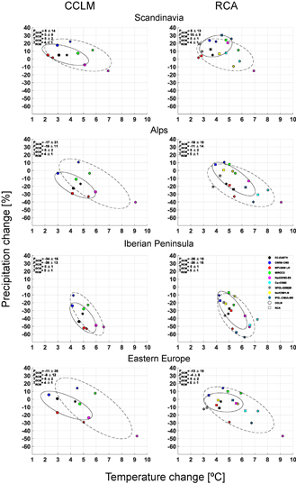
Figure 3. Climate change signal in the GCM and the GCM-RCM simulations. Panels show the bivariate climate change signal in terms of projected summer (JJA) temperature and precipitation changes for 2070–2099 versus 1971–2000 assuming the RCP8.5 emissions scenarios. The stars show the GCM results, and the circle (squares) the GCM-RCMs using the CCLM (RCA4). The colors indicate the driving GCM. The dashed (solid) line indicates the probability ellipse for the GCM (RCM) results, covering 68.2 % of the data. The mean precipitation (P, %) and temperature (T, °C) changes together with the standard deviations (mean ± σ), for the GCM and RCM ensemble, respectively, is given in the top left corner of each sub-figure.
Download figure:
Standard image High-resolution image
Next, consideration is given to projections from GCM-RCM model chains. According to the 'cascade of uncertainty' the uncertainty should increase when climate data from a GCM is regionally downscaled. Here we assess how the climate change signal is changing in the RCMs compared to the GCMs. Figure 3 compares the bivariate (near surface temperature and precipitation) climate change signals at the end of the century in the two RCMs versus the corresponding GCMs. Results for the summer season are shown for the same subdomains as in figure 2. The probability ellipse is calculated separately for the RCMs (full lines) and the GCMs (dashed lines) and spans one standard deviation of the data. Both the RCMs are substantially modulating the projected temperature and precipitation changes and are also reducing the model spread in terms of temperature and precipitation changes. The temperature change is substantially reduced by the RCMs compared to the GCMs, especially over Scandinavia, eastern Europe and the Alps, while over the Iberian Peninsula the temperature reductions by the regional models are not so strong. For GCMs that predict a comparatively low temperature change, the RCMs do not reduce the temperature change much, or may even increase it (as seen for the GFDL model for regions shown in figure 3).
The change in the precipitation is more complex, but there is a tendency of the RCMs to reduce the projected drying over the Alpine and Mediterranean regions, and to increase precipitation over Scandinavia, compared to the driving GCMs. The RCA model tends to increase the precipitation more than CCLM, as seen in particular over the Iberian Peninsula, the Alps and over Scandinavia. For a few GCMs the regional models are actually changing the sign of the projected precipitation change compared with the GCMs, consistent with previous studies conducted over different regions (Kjellström et al 2016, Mearns et al 2013, Zou and Zhou et al 2013).
4. Discussion
Since the resolutions of the GCMs are too coarse to provide adequate climate realizations on the regional scale, RCMs are commonly nested into GCMs to obtain more detailed descriptions of the regional climate. Even though this kind of dynamical downscaling has been used for almost three decades, there is still large skepticism. It has been stated that RCMs are merely producing 'uncertainty piled on top of uncertainty' (Kerr 2011), other studies argue with the 'garbage in, garbage out' paradigm, and it is often assumed that biases from the GCMs and RCMs are independent and thus the uncertainty should be increasing when the global data is translated into regional data, referred to as the 'cascade of uncertainty' (Wilby and Dessai 2010). In this study we are investigating the traditional dynamical downscaling method, where the RCMs are nested into GCMs to obtain more detailed descriptions of the regional climate. We have demonstrated that the two regional models RCA and CCLM yield a systematic reduction of the biases compared with the driving GCM.
What is behind the systematic reduction of the bias through the RCMs? As the effect is evident for both RCMs, which were developed independently and use two different sets of parametrization schemes (Kotlarski et al 2014), we believe that the improvement cannot be attributed to one single process or parameterization scheme, but likely derives from factors that in general distinguish the RCMs from the GCMs. There are two such factors: first, the RCMs considered have appreciably higher spatial resolution than the GCMs (here 50 km grid spacing versus on average 188 km for the GCMs considered). Second, while the GCMs are in general tuned in a way so that the global mean top-of-the-atmosphere energy balance matches observations (Hourdin et al 2016), RCMs are tuned or calibrated in current-climate simulations driven by reanalyses (Bellprat et al 2016, Rummukainen 2016). The prime target of the RCM tuning process is the performance of the RCM in terms of its regional distribution of surface temperature and precipitation.
To distinguish the role of the different parametrization schemes from the resolution effect, we performed an extra set of sensitivity experiments, where we decreased the horizontal resolution in CCLM to approximately 200 km (see the section 2 for details). With this setup, we downscaled two GCMs; one which shows a large temperature bias over several parts of Europe (MIROC5), and one with a lower bias (EC-EARTH). The results are presented in figure 2 and in the supplementary figures S2–5 (see diamond symbols). The CCLM corrects the GCM bias to a substantial extent, even at this coarse resolution. In some regions and seasons, the 200 km CCLM simulations are performing as well or even better than those with the 50 km horizontal resolution (e.g. figure 2(a)). These results suggest that it is not only the higher resolution that improves the RCMs compared to the GCMs, but that the set of parametrization schemes together with the regional tuning is indeed improving the performance of the downscaled climate data.
The two RCMs we have studied show a systematic reduction in the spread of the climate change projections compared to the driving GCMs (figure 3). The reduction in spread is thus not a surprising result, since there is an uneven comparison between the number of parametrization schemes in the GCM ensemble (one set of parameterizations for each GCM) and the RCM ensemble (the same set for all GCM-RCM simulations using the same RCM). If one RCM is downscaling several GCMs, the method is reducing the number of parametrization schemes: while all GCMs have different sets of parametrization schemes, this reduces to one set of parametrization schemes per RCM. That much of the model spread is related to the choice of parametrization schemes has previously been shown (García-Díez et al 2015). Nevertheless, both RCMs are modifying the climate change signal in a similar way, by lowering the GCM temperature projections. A similar effect has been noted when considering GCM and RCM simulations over Australia (Olson et al 2016).
The relation between summer temperature biases and projected temperature changes has been studied previously in GCMs (Christensen and Boberg 2012) and RCMs (Boberg and Christensen 2012), and it has been suggested that models with a warm temperature bias predict a stronger warming. We show here that the RCMs reduce the GCM biases and in the same manner lower the projected summer temperature changes. Previous studies have also argued that the common overestimation of interannual variability by GCMs in the observational period, with particularly large warm biases in warm summer months or seasons, could imply an overestimation of the climate change signal in the future (Buser et al 2009, Fischer et al 2012b, Kerkhoff et al 2015). On a process level, it has been argued that the temperature projections are overestimated due to incorrect representation of feedback mechanisms triggering enhanced drying (Bellprat et al 2013, Boberg and Christensen 2012). We thus suggest that one of the reasons for the reduced RCM biases and the lowered temperature projections in summer is that RCMs are better at representing near-surface processes that are important for reducing the drying feedback (e.g. a more realistic representation of boundary layer processes and the soil moisture's seasonal cycle).
We have focused on the summer season in four regions, but the other seasons and sub-regions show qualitatively similar results (see figures S2–8). There are only a few exceptions where the analyzed RCMs are not adding value to the GCM climate. Both RCMs tend to do a better job in correcting the GCMs when the GCM has a warm bias, compared to a cold bias. A predominantly cold bias in most seasons but particularly in winter, is a well-known deficiency in the EURO-CORDEX RCMs (Kotlarski et al 2014), which has been suggested to be related to topography (Kotlarski et al 2012) or convective and microphysical processes (Vautard et al 2013), or to the use of outdated aerosol climatologies (Bartók et al 2017, Zubler et al 2011, Schultze and Rockel 2017). This result emphasizes the need for continued model development. Moreover, even though we have only focused on the European domain, we would expect some improvements in other regions and for other models, particularly if the RCMs have undergone some regional tuning or calibration (e.g. Bellprat et al 2016).
5. Conclusions
In summary, the current study strongly supports the use of GCM-RCM model chains in regional climate change assessments. Our results show that the biases of the RCMs and GCMs are not additive and are not independent. The two RCMs systematically reduce the biases and modify climate change signals of the driving GCMs, even on scales that are considered well resolved by the driving GCMs. The results also suggest that the improvements are not exclusively due to the higher resolutions of the RCMs, but may also be due to different strategies in model tuning and calibration. While GCMs are tuned to represent the global energy and water balance (to provide global consistency of the simulated climate), RCMs are tuned to represent the regional climate (to provide an optimal representation of the regional processes). The results of the current study show that the combined GCM-RCM strategy is beneficial. Implicitly, our study also suggests that evaluating GCMs primarily with respect to their own near-surface climate may undervalue the quality of a GCM's circulation climate. We believe that our results are also applicable to the success of current numerical weather prediction systems, which in most regions rely on a combination of global and regional models.
In terms of European climate change projections, the RCMs imply a considerably weaker summer warming than the GCMs. The differences are most pronounced in eastern Europe, where the projections of the GCMs amount to about 6 °C, while the two RCM reduce this warming to between 4 and 5 °C (the mean changes are shown in figure 3). While the RCM- projected warming is 1 °C–2 °C smaller than from the GCMs, the anticipated warming still exceeds natural climate variability by a large margin (Fischer et al 2012b), and would thus likely have serious implications upon the incidence of heat waves and the availability of fresh water resources.
Acknowledgments
The CCLM climate simulations have been conducted at the Swiss Center for Scientific Computing (CSCS, Lugano) using resources from a PRACE allocation. Partial funding for this study has been provided by the Swiss National Science Foundation under Sinergia grant CRSII2 154486/1. The RCA simulations have been performed on computer resources provided by the swedish national infrastructure for computing (SNIC) at national supercomputer centre (NSC). Partial funding for this study has been provided by the Swedish MSB-financed project HazardSupport. We acknowledge the World Climate Research Programme's Working Group on Coupled Modelling, which is responsible for CMIP, and we thank the climate modeling groups (listed in table 1) for producing and making available their model output. We appreciate comments from Hansruedi Künsch and Reto Knutti on earlier versions of this manuscript. We thank Nico Kröner and Jan Rajczak for sharing programming codes and valuable discussions.
This study is dedicated to Daniel Lüthi who passed away at an untimely age in January 2018.
Footnotes
- *
Deceased.