

Abstract
Understanding the interplay between multiple climate change risks and socioeconomic development is increasingly required to inform effective actions to manage these risks and pursue sustainable development. We calculate a set of 14 impact indicators at different levels of global mean temperature (GMT) change and socioeconomic development covering water, energy and land sectors from an ensemble of global climate, integrated assessment and impact models. The analysis includes changes in drought intensity and water stress index, cooling demand change and heat event exposure, habitat degradation and crop yield, amongst others. To investigate exposure to multi-sector climate impacts, these are combined with gridded socioeconomic projections of population and those 'vulnerable to poverty' from three Shared Socioeconomic Pathways (SSP) (income <$10/day, currently 4.2 billion people). We show that global exposure to multi-sector risks approximately doubles between 1.5 °C and 2 °C GMT change, doubles again with 3 °C GMT change and is ~6x between the best and worst cases (SSP1/1.5 °C vs SSP3/3 °C, 0.8–4.7bi). For populations vulnerable to poverty, the exposure is an order of magnitude greater (8–32x) in the high poverty and inequality scenarios (SSP3) compared to sustainable socioeconomic development (SSP1). Whilst 85%–95% of global exposure falls to Asian and African regions, they have 91%–98% of the exposed and vulnerable population (depending on SSP/GMT combination), approximately half of which in South Asia. In higher warming scenarios, African regions have growing proportion of the global exposed and vulnerable population, ranging from 7%–17% at 1.5 °C, doubling to 14%–30% at 2 °C and again to 27%–51% at 3 °C. Finally, beyond 2 °C and at higher risk thresholds, the world's poorest are disproportionately impacted, particularly in cases (SSP3) of high inequality in Africa and southern Asia. Sustainable development that reduces poverty, mitigates emissions and meets targets in the water, energy and land sectors has the potential for order-of-magnitude scale reductions in multi-sector climate risk for the most vulnerable.
Export citation and abstract BibTeX RIS

Original content from this work may be used under the terms of the Creative Commons Attribution 3.0 licence.
Any further distribution of this work must maintain attribution to the author(s) and the title of the work, journal citation and DOI.
1. Introduction
The 21st century will see the global population increase from 7.5 billion in 2017 to an expected 8.5–10 billion in 2050 [1], with much of this growth in low- and middle-income regions. Future populations will be exposed to a range of climate change-related hazards of varying intensities and locations, with some 'hotspots' exposed to more risks than others, compounding the challenges [2–4]. Risks are not just dependent on the severity of climate change and subsequent hazards but critically depend on the population's spatial distribution (exposure) and their vulnerability and capacity to prepare for and manage changing risks [5]. Increasingly studies are showing that the world's poorest are disproportionately exposed to changes in temperature extremes [6, 7] and challenging hydro-climatic complexity [8–10]. In the water sector, between 8%–14% of the global population are expected to face severe reductions in available water resources between 1.7 °C–2.7 °C [11] and in the energy sector, more than 70% of a 'business as usual' 2050s population could expect climate sensitive changes in energy demand of +/− 5%, with negative impacts overwhelmingly in low and middle income countries [12]. Following ratification of the 2015 Paris Agreement, more work is required to understand the potential range of benefits of a 1.5 °C climate, what higher degrees of warming are projected to entail for different sectors [13] and to what extent people of different vulnerabilities will be impacted.
Along with other factors such as institutional governance, education, social structures and safety nets [14], vulnerability is strongly associated with wealth, although the wealthy in volatile climates are not immune [2]. Accounting for those that are 'vulnerable to poverty' were they to suffer a shock, like loss of employment or a climate hazard, is critical because much larger fractions of society exist in this precarious and transient state. In 2011, there were an estimated 767 million people living in extreme poverty with incomes of less than $1.9 USD/day, with a total of 4.2 billion (bi) classified as vulnerable to poverty living on $1.9–10 USD/day [15]. Escaping (or not falling back into) poverty, can be particularly difficult as the frequency of natural and climate hazards prevents asset accumulation [16] and impacts negatively on health, prices, productivity and opportunities [17]. The most optimistic scenarios, for example, project up to an 85% reduction in this vulnerable population to 616 million by 2050, with very good and sustained progress on the Sustainable Development Goals (SDGs).However in a high inequality scenario, the vulnerable population could remain as high as 4.0 billion in 2050 [18].
To understand the scale of this problem in the future, our objective is to assess the potential exposure of global and vulnerable populations to overlapping multi-sectoral hotspots. This work investigates how multi-sector risk changes with higher levels of warming and to what extent climate mitigation, socioeconomic development and poverty reduction can reduce risks. We use established methods [2, 4, 19] for aggregating climate risks, using 14 indicators across the water, energy, and land sectors (table 1, figure 1). We combine these indicators to produce multi-sector risk hotspot maps, compared for 1.5°, 2.0° and 3.0° changes in Global Meant Temperature (GMT) above pre-industrial conditions (figure 2). Critically, we investigate the exposure of the global and vulnerable population (income <$10USD/day) using three socioeconomic projections from the Shared Socioeconomic Pathways (SSPs 1–3) [20]. Our central scenario of sectoral risks is based on a 2 °C climate with 2050 population from SSP2. For the multi-sector hotspots, we assess the global and vulnerable exposure across SSPs and GMT change dimensions for 2050, to present insights in to the dynamics between socioeconomic development and risks at different levels of warming and to better understand the uncertainties.
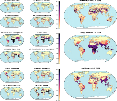
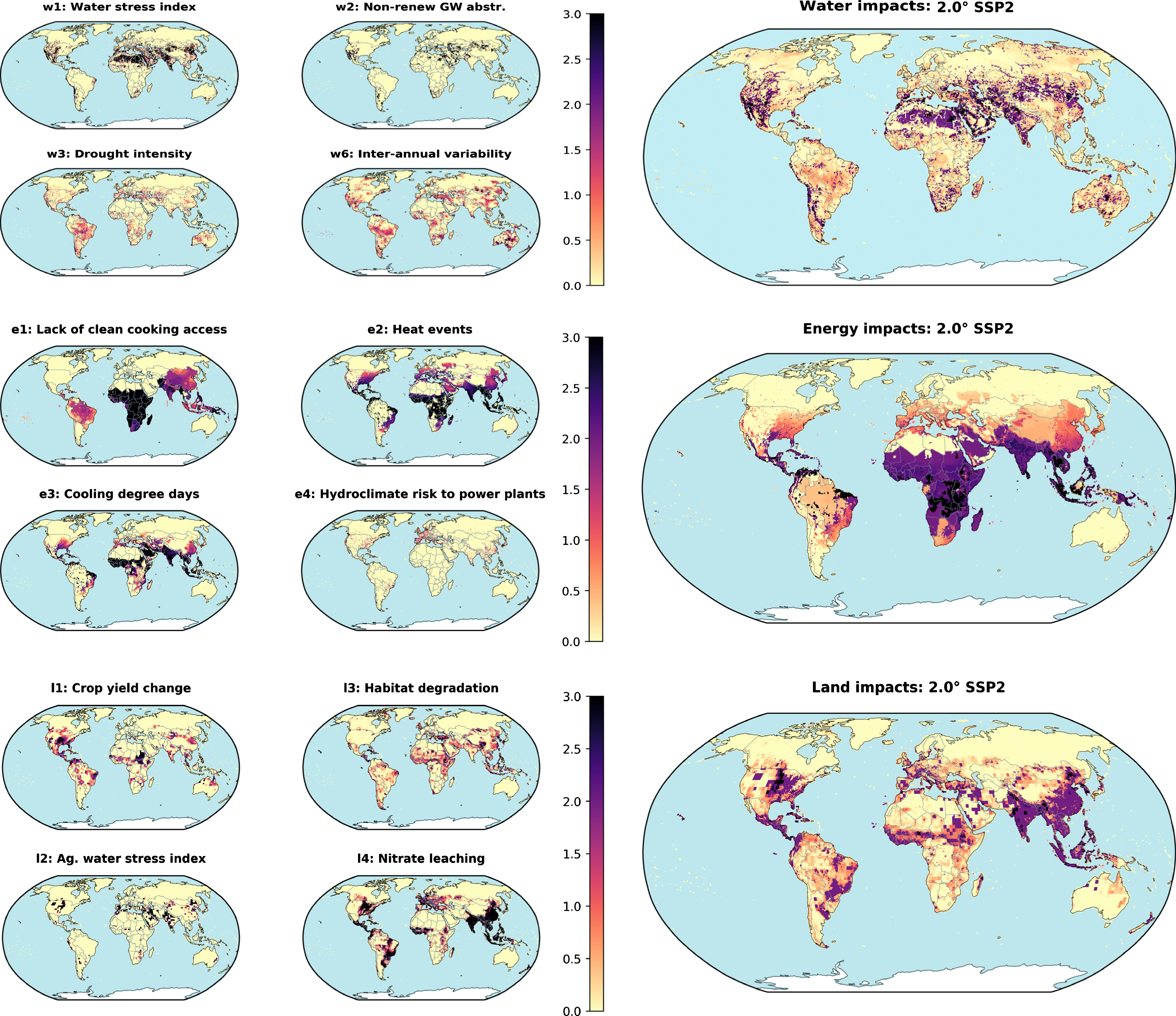
Figure 1. Sectoral score (0–3) maps for 2 °C GMT warming scenario. In the left column the individual indicators are shown, in the right column are the sectoral scores. Note that only four of the six water indicators are shown. Full indicator and sectoral exposure data available in SI tables S7–8.
Download figure:
Standard image High-resolution image
Figure 2. Multi-sector risk maps for 1.5 °C, 2 °C and 3 °C climates. Left column shows the full score range 0–9 (with transparency) and multi-sector risk score, MSR ≥ 5.0, in full colour. Right column greyscale underlay is the SSP2 2050 vulnerable populations, with the MSR ≥ 5.0 overlaid (only pixels ≥10 vulnerable persons km−2), indicating the concentrations of exposed and vulnerable populations (E&V). Moderate and high multi-sector impacts are prevalent where vulnerable people live, predominantly in South Asia at 1.5 °C, but spreading to sub-Saharan Africa, the Middle East and East Asia at higher warming.
Download figure:
Standard image High-resolution imageTable 1. Water, energy and land indicators and associated model combinations used in the study. GCMs are general circulation models, GHMs are global hydrological models. See Methods and supporting information (SI) for full details and references.
| Indicator | Description and methods | Models |
|---|---|---|
| Water | ||
| Water stress index | Water stress index (w1) as a fraction of net annual human-economic water demands (irrigation, industry, households) relative to available renewable surface water supply [42], as derived in the Water Futures and Solutions initiative [43]. | GCMs, GHMs |
| Non-renewable groundwater stress index | Non-renewable groundwater stress index (w2) is calculated as the fraction of total annual groundwater abstraction that is non-renewable (abstraction in excess of recharge) using data from Wada and Bierkens [44]. | HadGEM2-ES, PCR-GLOBWB |
| Drought intensity | Drought intensity (w3) change is calculated using daily river discharge deficit volume below Q90 over drought event duration, as derived in Wanders and Wada [45]. | 5 GCMs, 5 GHMs |
| Peak flows risk | Peak flows risk (w4) index is derived as locations where there is significant (50%+) ensemble agreement of a doubling or halving of the 20 year return period for river discharge, calculated using Generalized Extreme Value distribution fitting with a block-maxima approach as in Dankers, Arnell [46]. | 5 GCMs, 4 GHMs |
| Seasonality | Mean seasonality (w5) is the change in discharge seasonality index. Calculated as the coefficient of variation (standard deviation divided by the mean) of mean monthly discharge, it represents the variability of mean monthly discharge. | 5 GCMs, 5 GHMs |
| Inter-annual variability | Mean inter-annual variability (w6), is the change in discharge inter-annual variability index, calculated as the coefficient of variation of mean annual discharges, it represents the variability of mean annual discharge. | 5 GCMs, 5 GHMs |
| Energy | ||
| Lack of access to clean cooking | Lack of access to clean cooking (e1) fraction is projected from the reference energy scenarios for each SSP on a regional basis [47, 48], then downscaled using projected SSP Salamanca income distribution projections [18] by selecting the poorest population first within each country. | MESSAGE, SSPs, Salamanca |
| Heat event exposure | Heat event exposure (e2) is calculated as the sum of days from heat events lasting 3 or more consecutive days above the historical 99th percentile daily mean wet bulb air temperature. Only assessed at locations where Tmean p99 > 26 °C and population density > 10 persons km−2. | 5 GCMs |
| Cooling demand | Measure of the absolute growth in annual cooling degree days (CDD) (e3) with a set point temperature of 26 °C and population density > 10 persons km−2. | 5 GCMs |
| Hydroclimate risk to power production | Hydroclimate risk to power production (e4) index aggregates the combined hazard of four hydrological indicators, peak flows risk, drought intensity change, seasonality and inter-annual variability to a continuous hazard scale (as used with other indicators). This is multiplied by a capacity score according to the installed capacity in each grid square, using a global dataset of water-dependent thermal and hydro power plant capacity [49–51]. | 5 GCMs |
| Food and environment (land) | ||
| Crop yield change | Climate change impact on crop yield (l1) is estimated by the EPIC crop model under for ISIMIP future climate change scenarios [52] for 18 crops and 4 crop managements systems and overlaid with the distribution of crops and systems estimated by GLOBIOM land use model [53] for year 2000 [54] and aggregated across crops and crop management pixels (using calorie content). | 5 GCMs, EPIC + GLOBIOM |
| Agricultural water stress index | Agricultural water stress index (l2) indicates agriculturally-driven environmental water stress. By identifying locations where the monthly irrigated water demand are in excess of sustainable supply, it measures the fraction of environmental flow requirement (EFR) required to meet the agricultural demands [55–57]. | GLOBIOM + HadGEM2-ES + LPJmL |
| Habitat degradation | Habitat degradation (l3) is estimated as a % change from the share of land area within a pixel being converted from natural land to agricultural land (cropland and grassland) in the future as simulated by the GLOBIOM model [53, 58] and further downscaled to 0.5° [59]. | GLOBIOM + downscaling |
| Nitrogen leaching | Nitrate leaching from mineral fertilizer application over cropland (l4) is the flux of nitrate resulting from mineral fertilizer application to cropland and lost to surface water streams as simulated by EPIC [60] for 18 crops and crop management systems, and overlaid with GLOBIOM assumptions on future changes in crop yield and crop input use efficiency [61, 62] and downscaled GLOBIOM distribution projections of crop and crop management systems. | GLOBIOM + downscaling + EPIC |
1.1. Background on previous methods and assessments
Integrated assessment and impacts models use physical output variables from General Circulation Models (GCMs) to study specific sectors in more detail, for example in hydrology, land use and vegetation, energy and fisheries. [11, 12] GCMs and impacts models are frequently and consistently compared in model inter-comparison exercises, such as the Coupled Model Intercomparison Project (CMIP) [21] and the Inter-Sectoral Impact Model Intercomparison Project (ISIMIP) [22, 23]). Growing sectoral coordination means that model performance, results and uncertainty are more easily assessed within sectors, however there have been few multi-sectoral assessments to date [4, 24]. Research has brought together multiple indicators at different levels of GMT change, assessing the fraction of global land area impacted, for extremes of physical impacts [25] and for a wider range of impacts for multiple sectors [26]. Others have [27–29] similarly assessed risks, over various sectors with multiple indicators, but with little explicit analysis of where risks are projected to overlap.
To assess the severity of overlapping climate change risks, climate change indices and metrics on regional and national and gridded scales have been used using GCM variables such as precipitation, air temperature and sea-level rise [2, 19, 30–32]. And increasingly studies frame their results in terms of global mean temperature change as opposed to emissions scenarios. For example, Sedláček and Knutti [33] assessed 6 CMIP5 seasonal variables of the hydrological cycle for robust change [34], over 1 °C, 2 °C and 3 °C of GMT change, finding that over half of the world's current population will experience robust changes in precipitation, evaporation and relative humidity in a 2 °C climate. Similarly, Piontek et al [4] identified geographical overlaps of multisectoral exposure hotspots using single representative indicators for water, agriculture (four crop yields), ecosystems and malaria using sectoral thresholds to identify locations of 'severe' change.
Including different socioeconomic development pathways, which may be co-dependent on climate change mitigation, adds additional insight to future societal exposure and vulnerability. The Shared Socioeconomic Pathways [35–37] offer a comprehensive framework for joint consideration of socioeconomic development and climate change mitigation and adaptation challenges. New, socioeconomic projections with consistent 21st Century narratives are available for the SSPs for population [38], urbanization [39] and gross domestic product [40]. Additionally downscaled spatial population projections [41] and recent income distribution projections [18] enable new angles of climate impacts analysis that better represent exposure and vulnerability.
2. Methods
2.1. Framework overview
Building on the aforementioned approaches, this study: (i) developed indicator datasets at transient levels of GMT; (ii) applied score ranges to transform indicators onto common scoring scales; (iii) aggregated sectoral indicators to make sectoral score maps for water, energy and land; (iv) aggregated sectoral score maps to make multi-sector risk maps; and (v) combined multi-sector risk maps with population and vulnerable population projections to assess exposure and vulnerability to multi-sector risks.
We aim to examine simultaneously the change in physical exposures with projected evolution of population distribution and vulnerability to identify multi-sector vulnerability hotspots. This allows some evaluation of the three components of risk: hazards, exposure, and vulnerability [63].
The indicators are assessed across a range of global mean temperature rise relative to pre-industrial levels (1.5 °C, 2 °C and 3 °C), and population and economic activity trajectories consistent with the Shared Socioeconomic Pathways (SSP1, 2 and 3). The nine combinations thus span a wide range of potential outcomes but should not be viewed as equally likely or compatible. For example, it will be more difficult to reach ambitious climate targets in SSP3 as opposed to SSP1 and 2 because increased mitigation challenges are expected to accompany the slower development narrative of SSP3 [36, 64]. Thus, the sectoral results are mostly presented using the central scenario of 2 °C GMT with SSP2 in 2050, whilst sensitivities of GMT and SSP are explored in the multi-sector exposure results.
2.2. Selection of indicators and subsectors
Water, energy and land sectors were assessed across a set (Si) of 4–6 representative indicators (SI table S1 available at stacks.iop.org/ERL/13/055012/mmedia). Each indicator was processed to represent the change in hazard between future climatic conditions and the historical baseline (section 2.3). An exception is for the lack of clean cooking access indicator, as the availability of traditional biomass is not expected to change with climate change and any changes would be insignificant compared to the potential socioeconomic changes across SSPs. It is included as a key indicator of vulnerability (see SI table S2). Although not demonstrated in this study, the framework allows for the substitution and weighting of indicators, both within and between sectors, according to preferences of the analyst.
2.3. Climate forcing
Most indicator datasets in this analysis use as inputs the ISIMIP 'Fast Track' model database ensemble of five general circulation models (GCMs) from CMIP5 [21]: GFDL-ESM2M; HadGEM2-ES; IPSL-CM5A-LR; MIROC-ESM-CHEM; NorESM1-M. The GCMs were consistently downscaled to spatial resolution of 0.5°, bias-corrected [65] to observed data [66], and were selected for coverage of the uncertainty range in temperature and precipitation variables from the CMIP5 models [23].
We assess the climate hazards at three levels of global mean surface temperature (GMT) change: 1.5 °C, 2 °C and 3°C above the pre-industrial conditions (PiC), compared to a baseline period of 1971–2000, of ~0.6 °C above PiC (and acknowledging the importance of the PiC temperature choice [67]).These temperatures, possible at multiple timeframes within this century [68], do not represent climate stabilization scenarios, but are used to represent the risks at different levels of warming in a transient climate.
We follow the established time-sampling approach [4, 26, 69] of selecting a 30 year temperature timeslice, centred on the year at which the GCM passes the relevant GMT. GCM model runs are forced by the greenhouse gas and radiative forcing trajectories from the Representative Concentration Pathways (RCP) [70, 71], using RCP8.5 in the majority of cases and RCP4.5 and RCP6.0 in a few cases where the SSP-RCP combination is endogenous to the impact model (see SI table S1 for exact details). For example, HadGEM2-ES RCP8.5 passes 2 °C in 2028, so the 30 years selected to represent a 2 °C climate, were 2014–2043 inclusive.
To make meaningful and consistent comparison between the three GMT scenarios and three SSP socioeconomic projections, the year 2050 was chosen for the SSPs for scenario comparison. In this year, the three levels of GMT change (which are not stabilization scenarios) are all possible with varying probability, due to the range of emissions scenarios and geophysical response uncertainty [72, 73]. This was verified for consistency using the IPCC Working Group III scenario database (available online at: https://secure.iiasa.ac.at/web-apps/ene/AR5DB/) [74] (SI 1.2). This allows for a more consistent comparison of exposure, than a time-varying alternative, for example, which would be comparing 1.5 °C GMT change with a 2040s population and 3 °C with a 2080s population.
2.4. Indicator and sectoral aggregation
The indicators are combined in a consistent way to facilitate comparisons, impacts aggregation and to identify overlapping locations of risk. Whilst some studies use a single thresholds or discrete intervals [2, 4, 19, 30] for each sector, this binary approach potentially misses at-risk areas that may fall just under the threshold. Other studies used discrete intervals.
Our approach maps the sectoral impact indicators onto a continuous risk-indicator scale, ranging between no negative impact to high negative impacts and scored between 0 and 3. Intervals on the scale are specified by the sectoral modelling teams at [0, 1, 2, 3] to represent no, low, moderate and high levels of risk, as judged through interrogation of the original data, incorporating expert judgement, for which we test the sensitivity (section 2.5). The continuum between 0 and 3 can be linear or any other line (SI figures S4–5). Every gridsquare in each spatial indicator dataset is subsequently scored, Si, using the continuous scale. The scores are then aggregated to quantify a sectoral score, θs, for water, energy, and land, respectively.
For example, for the water stress index, it is commonly agreed that an index of between 0.2–0.4 represents water stress [42]. Thus, our central estimate uses 0.4 for a score of 3 (high risk), 0.3 for a score of 2 (moderate risk), 0.2 for a score of 1 (low risk) and 0.1 as threshold to get a score above 0.
For the aggregation of sectoral and multi-sector scores, in principle, either averaging or summation can be used. We use averaging for the calculation of the sectoral scores such that different numbers of indicators can be combined. Summation is applied then to the multi-sector risk calculation because using this aggregation to represent cumulative of risk is more intuitive.
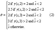
Sectoral scores are defined following two rules: first, the average score of all indicators per sector,  , is calculated. Second, in grid squares where a minimum number of sectoral indicators present at least a moderate or high risk, sectoral scores are assigned a minimum value. This is done to avoid the problem whereby moderate and high risk indicator scores get lost through averaging over multiple indicators.
Let γ be an operator that sums the number of indicators in the indicator function  with a score Si> τ.
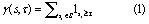
The sectoral score θ is adjusted following:
To calculate the aggregation of risk over multiple sectors, the sectoral scores (figure 1, central column) are summed (Σθ) to give the multi-sectoral risk score (M) that combines all indicators on a scale of 0–9. In this way, we assess the aggregation of risk over multiple sectors.
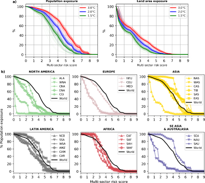
Figure 3. Distributions of global population and land area exposure to multi-sector risk score in 2050 with SSP2 population. Top panel (a) shows the exposure aggregated for the whole world by population and land area. Shaded areas around the lines represent the indicator score ranges uncertainty (Methods 2.5, and SI 1.4). Lower panel (b) is the population exposure for over 27 IPCC land regions (SI table S4 for three letter region codes). Noticeably, the differences in MSR on population, according to GMT, are most pronounced when MSI ≈4.0. At this level, population exposed in 1.5 °C is less than half that of a 3 °C climate. Land area exposure differences are smaller, as some of the impacts indicators are more driven by population. The differences between regions (b) are substantial, for example all North American subregions are below the global median exposure, whilst almost all Asian regions are above.
Download figure:
Standard image High-resolution image2.5. Indicator score ranges and uncertainty
Given disagreement and uncertainty on how to determine the score scales, score ranges specify low (precautionary), central and high (conservative) estimates for each point on each indicator scale (SI table S4). Each sectoral modelling team from the IIASA Water, Energy and Ecosystems Services and Management research programs reviewed and justified the score ranges for each indicator. Our sensitivity analysis ran 100 realisations, where for each indicator, the interval was sampled randomly from the uniform distribution of the score ranges (SI figure S5). Percentiles of these expert-informed score-ranges are subsequently used in the uncertainty analysis (figure 5, also evident in figure 3(a)).
2.6. Component uncertainty analysis
Our uncertainty analysis [75] determines the variability (through coefficient of variation) across the key uncertainty components of GCM, Impact Model, Score Range, GMT and SSP (figure 5). This was systematically assessed using all available model variants and scenarios (290 in total, hereafter variants) by counting the number of gridsquares with a score above the moderate risk threshold (in all cases Si ≥ 2, apart from the hotspot score Msi ≥ 4), with the coefficient of variation calculated across that component. This assessment was carried out at three exposure subsets (SI figures S25–27): all land gridsquares (~65 000); gridsquares with population density > 10 people km−2 (~21–23 000, depending on SSP); gridsquares with vulnerable population density > 10 people km−2 (~5–12 000).
2.7. Socioeconomic pathways, income projections and gridded vulnerability
Gridded projections of population and GDP for SSPs 1–3 spanning 2010–2050 [41] at 0.125° resolution are used to identify the distribution and numbers of exposed and vulnerable populations. We use recently compiled datasets of global income distributions and inequality [18] to estimate vulnerable populations using an income threshold. These datasets are generated for each scenario using machine-learning regression tree techniques for urban and rural income, which are downscaled using urbanization and migration patterns to give gridded projections of vulnerable population (SI section 3.1, figure S15).
This analysis uses definitions from the World Bank for categorising population as vulnerable. Whilst income level of $1.9 USD/day (2011 purchasing power parity) commonly defines extreme poverty, those living on <$10 USD/dayare considered vulnerable to poverty. This category and income level is appropriate because it specifically captures the population fraction that lack 'economic stability and resilience to shocks that characterizes middle-class households' [76, 77]. These shocks can be natural hazards, loss of income, illness or conflict, for example.
2.8. Multi-sector hotspot threshold analysis
Whilst the hotspot analysis uses a continuous distribution of impacts scoring, thresholds are used to cut the population exposure according to multi-sector risk (MSR) severity and population vulnerability.
Specifically, we consider that MSR ≥ 4.0 defines a multi-sector risk (see 3.2 for explanation). The total exposed and exposed and vulnerable populations decrease with higher MSR thresholds. For the central case, we use MSR ≥ 5.0 to indicate a multi-sector hotspot, with sensitivity results at MSR ≥ 4.0 and MSR ≥ 6.0 in the SI. The additional population exposed at 2 °C and 3 °C, above the 1.5 °C reference case, is presented in SI figure S24.
3. Results
We first present the sectoral indicator results, followed by the multi-sector risks, and finally the exposure and vulnerability assessment on global and regional basis.
3.1. Sectoral results
Water sector indicators have a wide range of risks of varying spatial coverage. Results are driven both by small areas of concentrated, high score indicators (w1, w2, w4) and widespread areas of moderate risk (w3, w5, w6). Water stress (WSI) and groundwater stress indices are substantially demand driven and thus are spatially concentrated in population centres and intense water demand regions. The more bio-physical indicators of drought intensity, inter-annual variability, and seasonality have more widespread risks and affect larger areas of land, including cropland and less populated areas. Arid areas for indicators w3 to w6 were masked out. Areas of particular concern include southwestern North America, southeastern Brazil, northern Africa, the Mediterranean, the Middle East, and western, southern and eastern Asia.
The energy sector indicators are strongly driven by locations of higher air temperatures and population density, due to the expected increases in air temperature changes that drive cooling energy demands and heat event exposure, particularly in the tropics. The hydroclimatic risk to power plants indicator is confined to a very small proportion of land grid squares (6%); however, high correlation of power plants with population density means the effects are not lost when accounting for population exposure. Few locations by spatial extent present high levels of risk, aside from the Middle East, pockets of sub-Saharan Africa and Southeast Asia, driven by low clean cooking access, more heatwaves and higher cooling demands. Large areas present consistently medium levels of risk, such as sub-Saharan Africa, central, South and Southeast Asia and central America.
Land sector impacts are widespread and cover large portions of all continents except Australia. Nitrate leaching is most widespread with many locations exceeding sustainable levels due to agricultural input intensification. Reductions in crop yields and habitat degradation also drive the sectoral score. Locations of agricultural water exploitation that would violate environmental flow requirements, increases in areas already dependent on irrigated agriculture: North America, South Asia, and China. Overall, Midwest United States, southeastern Brazil, Ethiopia and South Sudan, the Mediterranean and most of South and Southeast Asia, all present moderately high impacts.
3.2. Multi-sector climate risks and global exposure
Multi-sector risk (MSR) occurs at locations where two or more sectors surpass a tolerable level of risk. In this study, we consider that the minimum MSR to define a multi-sector risk is 4.0. It represents, for example, two sectors at moderate risk (2 + 2), one sector at high risk and another at low levels (3 + 1), three sectors at low-moderate risk (e.g. 3 × 1.34), or a similar combination. MSR ≥ 6.0 represents moderate risk across 6+ indicators in three sectors, or high risk in 4+ indicators in two sectors. An MSR of 9 is the theoretical maximum score for any grid square, which following the hotspot scoring would indicate at least two indicators in every sector at high risk, fortunately not observed in these results. Here, we present results at an MSR ≥ 5.0, with sensitivity at 4.0 and 6.0 (SI figures S12–14, S16–21).
For the multi-sector risk scores two main trends emerge as global mean temperature rises (figure 2). First, the area of land affected by climate risks grows in area, particularly populated areas (figure 2, figure 3(a)). At 1.5 °C risks are predominantly in South Asia. Secondly, the risks intensify in some locations, with more MSR heterogeneity and more pronounced differences between the 1.5 °C and 3 °C scenarios, as shown by the wider distribution in figure 3(a). For example, at 1.5 °C, MSR scores between 4–6 are fairly uniform across small areas, whilst a 3 °C GMT results in hotspots of high MSR, interspersed with wider areas of moderate risk. High risks occur primarily in Central America, East Africa and West Asia, the Mediterranean, the Middle East, most of South Asia and East China.
Although the fraction of global land area exposed to MSR ≥ 5.0 is 3%–16% across GMT scenarios, the equivalent fraction of exposed population is substantially larger and rises more rapidly with GMT increases (figure 3(a)). For example, whilst at 1.5 °C only 16% (1.5bi) of the population faces MSR ≥ 5.0, 29% (2.7bi) and 50% (4.6bi) are similarly exposed in 2 °C and 3 °C climates, respectively. These impacts also scale with latitude, noticeably between 40°N and 10°S (SI 3.4).
Comparing the macro-regions (figure 3(b)), Latin America, Africa and Southeast Asia and Australasia include at least one region with worse population exposure than the global median (Caribbean, West Africa, Southeast Asia). The exceptions are Asia, where most regions are above the global median exposure, and North America and Europe, where all have lower than median exposure. The least exposed region is Alaska and the most exposed regions are Southeast Asia, South Asia and Tibetan Plateau.
3.3. Global exposure and vulnerability
Considering the total global population exposure (MSR ≥ 5.0), global mean temperature rise has a considerably stronger effect than the differences in population between the SSPs. Between 1.5 °C and 2 °C, the total population exposure to multi-sector risks increases by 69%–113% (SSP3-SSP1), whilst the level of exposed and vulnerable population (E&V) (black shaded areas figure 4(a)) increases by 60%–258% (with large differences in absolute numbers between the SSPs (SI figures S16–18, tables S6–7)). At 3 °C, whilst impacts are more severe, the number of E&V increases by similar absolute numbers, but less in relative terms. This is largely because the spatial extent of risks does not increase as much between 2 °C–3 °C as it does from 1.5 °C–2 °C (figure 2). Furthermore, whilst at 1.5 °C, locations may experience only moderate-high impacts in one sector, at 2 °C there is a strong emergence of multiple, moderate-high risks.
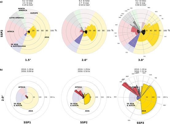
Figure 4. Global population exposure and vulnerability. Upper row (a) background is the total global populationin 2050 for SSP2, whilst in the foreground, the fraction of exposed population (MSR ≥ 5.0, strongcolours). Black shaded central segments are the exposed and vulnerable (E&V) population. For global exposure, GMT is the dominant driver over SSP population. However, the lower panel (b) shows how important socioeconomic development is for reducing the E&V population. It compares, for a 2 °C climate, the E&V population in 2010 (background circle, currently 4.2billion), compared with the projected E&V population in 2050 in the foreground. Whilst poverty reduction in SSP1 almost eradicates the E&V population in most regions by 2050, SSP3 results in substantial increases compared to 2010 in Asia and Africa due to high levels of inequality.
Download figure:
Standard image High-resolution image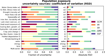
Figure 5. Contributions to uncertainty, measured as coefficient of variation (relative standard deviation, RSD), on proportional and absolute basis for gridsquares with exposed (indicator/sectoral/MSR scores ≥ 2/2/4, respectively).
Download figure:
Standard image High-resolution image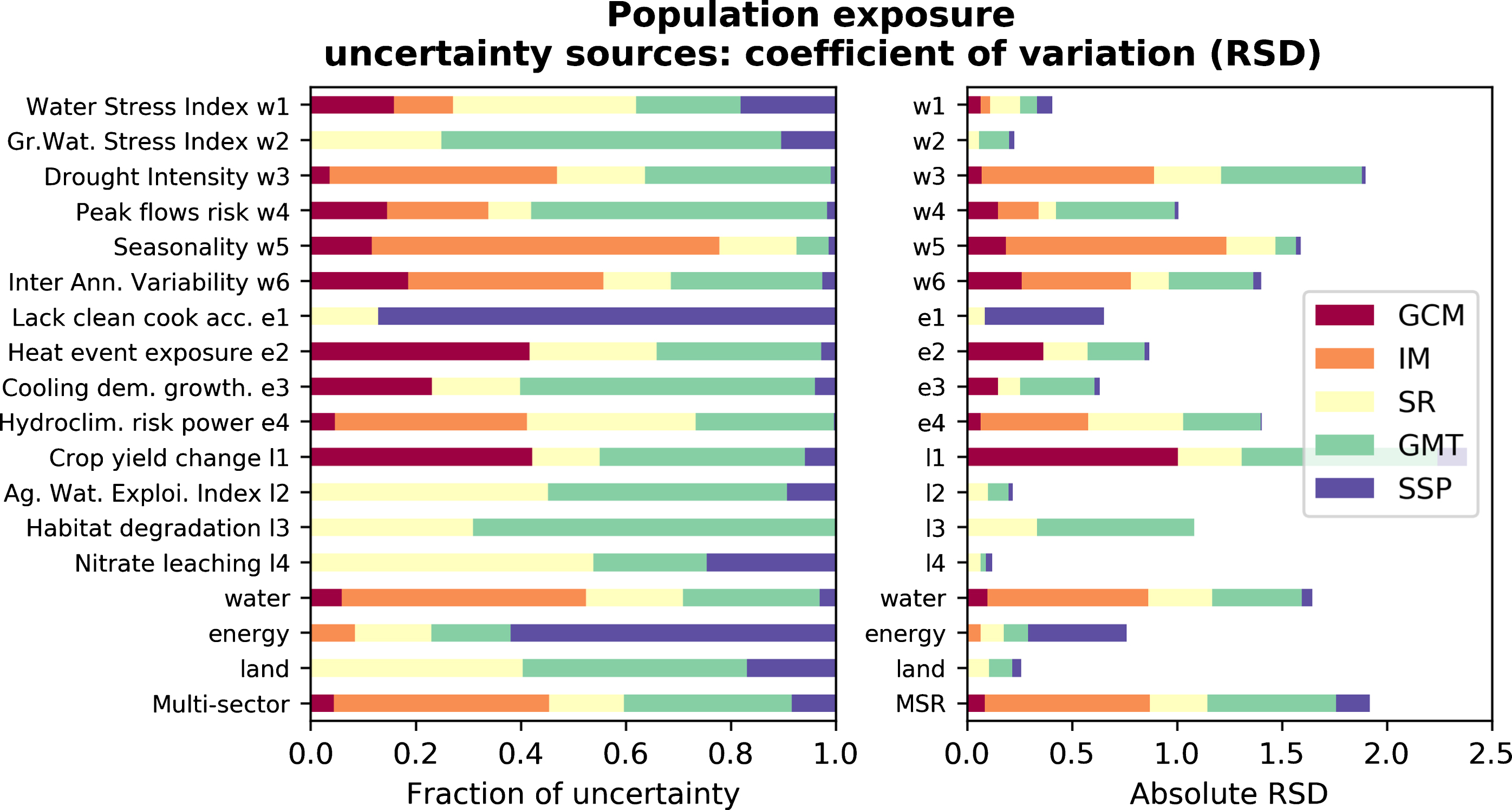
The benefits of poverty and inequality reduction are made clear when E&V population numbers are compared for different SSPs (figure 4(b)). Whilst SSP1, and to a large extent SSP2, project widespread poverty reduction primarily across Asia and Africa, in SSP3 poverty and inequality scarcely improves by 2050. What is achieved in Southeast and East Asia is offset by growing poor populations in Africa and South Asia. South, East and West Asia, have both some of the highest MSR scores and vulnerable populations (figure 3). Subsequently, in SSP3 there are between 8–32x more E&V population compared to SSP1, concentrated in the African and Asian regions with between 25%–100% more E&V in 2050 than compared to the 2010 demographic.
The largest co-benefits of poverty reduction and climate mitigation are for Africa and South Asia. Overall, there are approximately factors of ~30–190x difference of total E&V population between the best case (SSP1/1.5 °C) and worst case (SSP3/3 °C) scenario combinations: with more severe impacts (i.e. MSR = 6.0) the differences are accentuated (SI figures S16–21, tables S6–7). This growing scale factor with MSR threshold indicates that in worst case scenarios, higher fractions of a larger vulnerable population will be living in areas of particularly high risk.
Latitude also plays a role in the distribution of impacts (SI figure S23), consistently across a number of metrics. Whether assessed by mean score per pixel, cumulative score, land area-weighted or population-weighted impact, latitudes between 40°N to the equator fare worst; southern hemisphere quite poorly; and north of 40°N above average.
4. Discussion
Sustainable development that actively reduces socioeconomic inequality, poverty and population growth in Africa and Asia is ultimately the most effective way of reducing the total number of people categorized as exposed and vulnerable to climate change risks. An SSP3 future, with which low emissions scenarios are technically incompatible, results in order of magnitude higher exposed and vulnerable populations than SSP1. However, keeping population and inequality levels as low as projected in SSP1 is extremely ambitious and only possible if SDG targets for mortality, reproductive health and female education are achieved and sustained long-term [78].
Even still, the huge absolute numbers of people exposed to multi-sector risks (~1–5 billion), even in high income countries, underscore the benefits of climate mitigation. Most strikingly, the differences between 1.5 °C and 2 °C are substantial, strongly indicating the compounding risk with higher levels of warming. Efforts to meet the SDGs and low temperature targets of the Paris Agreement will substantially reduce global exposure to multi-sector risks, especially if recognized co-benefits are targeted [79]. Energy sector targets will facilitate achievement of other SDGs, particularly climate [80–82]. Without action on climate change (SDG13), including slowing the rate of warming, achieving the goals for water, energy, food and land (SDGs 6, 7, 2 and 15), amongst others [83], will be more difficult. Similarly, almost all the SDGs are likely to contribute to poverty eradication (SDG1) and climate action (SDG13). Additionally the work may support other multi-lateral environmental agreements, such as the Sendai framework on disaster risk reduction and the Addis Ababa Agreement on finance and investment for sustainable development.
Hotspots with high multi-sector risk, such as in West Africa, South and Southeast Asia, the Middle East, and north east Brazil, indicate where vulnerable populations will benefit most from targeted actions and further modelling exercises [85]. Further assessment could also include a broader coverage of sectors and indicators, for example, coastal and marine environments and health, or analysis at river basin and country scales.
In selecting indicators, understanding both their correlation (SI figure S28) and uncertainty structure (figure 5) has contributed to important analytical improvements and interpretation of the results. Whilst model and internal uncertainties (from GCM, Impact Models (IM) and Score Range (SR)) contribute most to impact uncertainties over land, irreducible scenario uncertainty (GMT and SSP) becomes significantly more important in every indicator when assessing exposed and vulnerable populations. Notwithstanding, improving model performance in highly populated regions is critical. Whilst the uncertainty analysis indicates that uncertainties in the water indicators are largest, it was also the sector with the largest model ensembles, with up to 25 GCM x IM combinations. The covariance analysis revealed generally very low correlation between indicators, particularly in populated areas, indicating that the resulting challenges will need multiple strategies, as opposed to tackling key pairs of highly co-dependent indicators. Further work could consider the risks of specific combinations of dependent variables, such as for heat events, drought and crop-yields, using multivariate approaches for compound extremes, because univariate approaches can underestimate these risks [86].
It is not just extremes that result in the most severe impacts. Average events can have extreme impacts because of high vulnerability, antecedent conditions and low coping capacity [14]. Low incomes, informal employment and low property values are poorly represented by traditional loss accounting approaches and indicators like loss in GDP [87], cost-benefit analysis and damage functions. This can result in gross underestimates of the economic and social impacts on the most vulnerable in society. Whilst the use of a global income level to represent vulnerability is a simplification, nonetheless, this assessment is the first to use gridded projections of income distribution to indicate future vulnerability at the global scale. Analysis using different income levels, or national and provincial poverty lines and at urban-rural gridded disaggregation will soon be possible and will provide even better insights on how risks could be spatially distributed in the future.
5. Conclusions
Although global exposure to multi-sector risks (figure 3) will affect a relatively small fraction of global land area, the risks to human populations will be large. Between 1.5 °C–3 °C, the increase in exposed population to multi-sector risks almost doubles from 1.5 °C–2 °C, and similarly again at 3 °C (1.5:2.7:4.6 bi). The differences between the socioeconomic projections are smaller, but not insignificant and are due to different population numbers. Both the scale of and the differences between these numbers underlines the multi-dimensional risks of climate change that will be experienced across the world regardless of wealth.
Exposure in Asian regions is the most severe, on proportional and absolute terms, due to the high concentrations of population and the high multi-sector risks of those regions. Asian and African regions face high proportions (>75%) of exposed population compared to their total population.
For populations exposed and vulnerable to poverty (E&V), i.e. daily income<$10/day, the importance of socioeconomic development potentially alters the number of E&V by an order of magnitude (~0.1–1.5bi, SSP1–3). Whilst approximately 85%–95% of global exposure falls to Asian and African regions, they have 91%–98% of the E&V population, approximately half of which in South Asia.
As the most undeveloped region, Africa fares worse than most regions (particularly East Africa), especially in high inequality socioeconomic scenarios and high warming climate scenarios. In higher warming scenarios, African regions have higher fractions of the global E&V population, ranging from 7%–17% at 1.5 °C, doubling to 14%–30% at 2 °C and again to 27%–51% at 3 °C.
The results also indicate that the poorest are also disproportionately impacted by multi-sector risks. Compared to a 1.5 °C baseline, the number of exposed and vulnerable scales faster than the exposed population, driven by both the warming level and the inequality levels. Further assessments to understand the distributional risks of climate change to different levels of vulnerability are required.
Climate mitigation alone is not enough to reduce exposure to the world's poorest, who will still be vulnerable to impacts at 1.5 °C. Action to rapidly reduce inequality, eradicate poverty and promote proactive adaptation through mechanisms such as the SDGs, would greatly reduce the size of exposed and vulnerable population, especially if co-benefits for climate mitigation also accrue.
Acknowledgments
The authors acknowledge the Global Environment Facility (GEF) for funding the development of this research as a part of the 'Integrated Solutions for Water, Energy, and Land (ISWEL)' project (GEF Contract Agreement: 6993), and the support of the United Nations Industrial Development Organization (UNIDO). Additionally, we acknowledge the ISIMIP Project and community, from which some of this work's raw input data is derived, as well as technical assistance that has been provided. EB acknowledges funding from his IIASA Postdoctoral Fellowship, Daniel Huppmann and Oliver Fricko for advice, Catherine Raptis for assistance with power plant datasets and the Python xarray development team for software support [88].