

Abstract
Analysis systems incorporating atmospheric observations could provide a powerful tool for validating fossil fuel CO2 (ffCO2) emissions reported for individual regions, provided that fossil fuel sources can be separated from other CO2 sources or sinks and atmospheric transport can be accurately accounted for. We quantified ffCO2 by measuring radiocarbon (14C) in CO2, an accurate fossil-carbon tracer, at nine observation sites in California for three months in 2014–15. There is strong agreement between the measurements and ffCO2 simulated using a high-resolution atmospheric model and a spatiotemporally-resolved fossil fuel flux estimate. Inverse estimates of total in-state ffCO2 emissions are consistent with the California Air Resources Board's reported ffCO2 emissions, providing tentative validation of California's reported ffCO2 emissions in 2014–15. Continuing this prototype analysis system could provide critical independent evaluation of reported ffCO2 emissions and emissions reductions in California, and the system could be expanded to other, more data-poor regions.
Export citation and abstract BibTeX RIS

Original content from this work may be used under the terms of the Creative Commons Attribution 3.0 licence.
Any further distribution of this work must maintain attribution to the author(s) and the title of the work, journal citation and DOI.
Fossil fuel combustion is the primary cause of increasing atmospheric CO2 concentration and associated radiative forcing [1]. Over 1990–2014, CO2 emissions from fossil fuel combustion and cement production (ffCO2) are estimated to have increased by ~60% globally [2] but by only ~9% in the United States [2]. The 2015 Paris Agreement of the UN Framework Convention on Climate Change adopted greenhouse gas mitigation pledges from individual countries [3], and many other mitigation policies are being implemented on the subnational scale. California's Global Warming Solutions Act of 2006 and subsequent policies set out to progressively reduce greenhouse gas emissions to meet targets for 2020 and 2030, with extensions planned for 2050.
'Bottom-up' estimates of CO2 emissions from fossil fuel combustion and cement production are based on calculations using data on fuel production and usage, carbon content of fuel, combustion efficiency of sources, and information on individual emitting activities [2, 4]. California's in-state fossil fuel CO2 emissions in 2014–15 were 91 million tonnes of carbon per year (MtC yr−1), with another 26 MtC yr−1 emitted by out-of-state electricity production, the military, and interstate and international shipping and aviation [4]. Fossil fuel CO2 emissions from California are about 1% of the global total.
Bottom-up calculations of fossil-derived CO2 (fossil fuel CO2 or ffCO2) emissions have historically been regarded as having relatively small uncertainties, and natural carbon fluxes often produce stronger spatial and short-term variations in atmospheric CO2. Therefore, 'top-down' studies of atmospheric CO2 incorporating atmospheric measurements and modeling have historically focused on natural carbon fluxes including photosynthesis and respiration [5, 6]. However, recent work has shown there can be large differences in national fossil fuel CO2 emissions estimated by different groups [7, 8], and uncertainties in emissions are much larger at sub-national scales [9, 10]. These discrepancies suggest that top-down studies incorporating the measurement of a tracer that distinguishes fossil-derived CO2 (ffCO2) could be useful for evaluating ffCO2 emissions on regional scales [11].
Top-down studies for ffCO2 emissions are still in the early stages of development [12–15], in comparison to relatively well-developed applications of top-down emissions estimates for other greenhouse gases such as methane [16, 17] and hydrofluorocarbons [18] that have revealed biases in corresponding bottom-up estimates, which tend to have large uncertainties. Top-down studies estimate the distribution and magnitude of emissions that minimizes differences with observations, typically also minimizing the deviation from a prior estimate of emissions following Bayesian statistics. Estimates of the spatial distribution of ffCO2 emissions have been produced using data from large point sources such as power plants and allocating other emissions using proxy data such as population, road networks or light observed at night by satellites [10, 19, 20], which can be used for prior emissions estimates in top-down studies (figure 1).
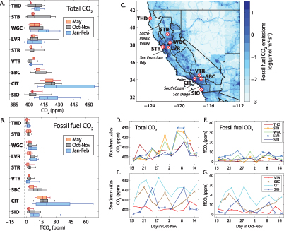
Figure 1. Observations of CO2 and ffCO2 from the California network. Observations for each site shown by quartile using boxplots for (A) total CO2 concentration and (B) ffCO2 concentration. The three campaigns conducted in 2014–15 are shown in different colors. Sites are ordered vertically according to location. The full range for total CO2 at CIT in January–February is 409–476 ppm. (C) Annual mean ffCO2 emissions from Vulcan v2.2(19) within the US for 2002 and from EDGAR v4.2 FT2010(29) outside the US for 2008. The sites in the observation network are shown as circles on the map: Trinidad Head (THD), Sutter Buttes (STB), Walnut Grove (WGC), Sutro (STR), Sandia-Livermore (LVR), Victorville (VTR), San Bernardino (SBC), Caltech (CIT) and Scripps Inst. Oceanography (SIO). Lines show the boundaries of the 16 subregions of California used in the inversion, with four major regions labeled. Individual observations conducted approximately every 3 d are shown in (D)–(G) for the October–November campaign. Total CO2 concentration is shown in (D) and (E) and ffCO2 concentration is shown in (F) and (G) for Northern California sites and Southern California sites separately. Uncertainty in ffCO2 is approx. ±1.5 ppm, indicated by the vertical dashed lines in (B).
Download figure:
Standard image High-resolution imageWe conducted a field study to observe ffCO2 with high spatial and temporal resolution over the state-wide California region using radiocarbon (14C) as a fossil fuel tracer, and to use the observations in a top-down calculation of California's ffCO2 emissions. Unlike previous studies of 14C-based ffCO2 observations that have focused on individual urban areas [11, 21, 22], we expanded the observational network to the regional scale in California, a political region that is implementing greenhouse gas emissions reduction policies.
Measurements of 14C in CO2 distinguish CO2 added by fossil fuel combustion and cement production because 14C has a half-life of 5700 years and million-year-old fossil fuels have lost all 14C to radioactive decay. The ratio 14C/C in CO2 is therefore reduced by the addition of CO2 from fossil fuel combustion, and measurements of 14C/C can be used to quantify ffCO2 [23]. Measurements of the ratio 14C/C are reported as Δ14C, in part per thousand (‰) deviations from a standard ratio [24]. Estimates of ffCO2 do not include anthropogenic CO2 emissions from non-fossil sources such as wood or biofuel burning.
Measurements of CO2 concentration and Δ14C in CO2 were conducted at nine existing observation sites across California and used to calculate ffCO2 with uncertainty of ±1–1.9 ppm (1-σ) (detailed methods, figure 1(A), table S1 available at stacks.iop.org/ERL/13/065007/mmedia). The network includes the urban regions of Los Angeles, San Francisco, Sacramento and San Diego as well as other parts of the state, with coastal stations sampling 'upwind' or 'background' composition during certain conditions. The observation network covers spatial scales of approx. 0.4 million km2 and the flask-based observations of ffCO2 are sensitive to regional emissions occurring over timescales of several days. The sampling strategy enabled the observation of different seasons, meteorological conditions and days of the week by collecting samples every 2–3 days at 14:30 Pacific Standard Time during three month-long campaigns in different seasons: May 2014, October–November 2014 and January–February 2015. Sampling was conducted in the afternoon to sample well-mixed conditions [25] that are most representative of large-scale influences and best simulated by atmospheric transport models.
Observed CO2 concentration in the flask samples ranged from 395 ppm to 431 ppm at non-urban sites (THD, STB, WGC, VTR), and from 395 ppm to over 480 ppm at urban sites (CIT, SBC, STR, LVR, SIO) (figure 1(B)). ffCO2 concentration derived from Δ14C observations ranged from approx. 0–14 ppm at non-urban sites and from approx. 0–68 ppm at urban sites, with the highest values observed at CIT in January–February (figure 1(B)).
Temporal variability in ffCO2 is shown by the range of ffCO2 in figure 1(B) and by the individual ffCO2 measurements in figures 1(F) and (G). The observed ranges in total CO2 concentration are larger than the observed ranges in ffCO2 concentration at each site, indicating that CO2 exchange with terrestrial ecosystems contributes to observed CO2 variation across California (figure 1), even at urban sites. For most sites, ffCO2 can vary from near zero to more than 5 ppm from day to day, reflecting variations in meteorological conditions. In particular, 'Santa Ana' conditions exhibiting high pressure over the Great Basin and off-shore winds were observed November 4–9, associated with relatively high ffCO2 at several sites including SIO, STR, LVR and WGC (figure 1, figure S1). Median ffCO2 is higher in winter at most sites due to seasonal changes in atmospheric transport.
Simulations of ffCO2 at the sites and times of the observations were conducted with the Vulcan v2.2 fossil fuel emissions estimate [19] for 2002 and the Weather Research and Forecasting—Stochastic Time-Inverted Lagrangian Transport (WRF-STILT) atmospheric model [26] with nested domains having spatial resolution of 4 km across California and 1.3 km in urban regions, following Fischer et al [2, 5, 27]. We use emissions from 2002 because detailed state-wide emissions estimates with hourly temporal resolution and 10 km spatial resolution are only available from Vulcan for 2002. Emissions in California were estimated to decrease by 8% from 2002 to 2014–15 [4]. For fossil fuel emissions outside of the US, we use annual mean estimates from EDGAR v4.2 FT2010 [28] for 2008.
Differences between simulated and observed ffCO2 are within the ±1.5 ppm (1-σ) nominal measurement uncertainty for 92 of 205 samples (45%), and within ±3.0 ppm (2-σ) for 135 of 205 samples (66%). Across all samples, observed ffCO2 is higher than simulated ffCO2 in more samples (136 samples) than observed ffCO2 is lower than simulated ffCO2 (69 samples). The largest differences are found at LVR and SBC in January–February, and at CIT in May (figure 2).
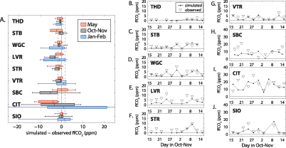
Figure 2. Comparisons between ffCO2 in simulations and observations. (A) The difference between simulated ffCO2 and observed ffCO2 for each site and each field campaign in 2014–15, plotted using boxplots similarly to figure 1. Simulations here use the prior Vulcan v2.2 time-varying ffCO2 emissions estimate [19]. The full range for CIT in January–February is −30 to +51 ppm. The vertical dashed lines show the typical ffCO2 measurement uncertainty of ±1.5 ppm (range of ±1.0 to ±1.9 ppm). (B)–(J) Simulated and observed ffCO2 for each site during the October–November 2014 campaign. Similar plots are shown for all campaigns in figure S2. Measurement uncertainty in ffCO2 is similar to the symbol size in (B)–(J).
Download figure:
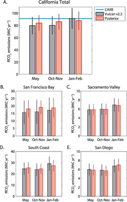
Standard image High-resolution imageIncorporating the observed and simulated ffCO2 into Bayesian inverse estimates of ffCO2 emissions following Fischer et al [27], we find that California in-state total ffCO2 emissions are 83.8 MtC yr−1 for May, 85.9 MtC yr−1 for October–November and 87.7 MtC yr−1 for January–February with 95% confidence intervals of ±13 to ±15 MtC yr−1 (table 1, figure 3(A)). These 'top-down' inverse estimates use the time-varying Vulcan v2.2 emissions estimate as a prior estimate of emissions, and then adjust the emissions in 16 individual subregions of California (figure 1) and one additional region incorporating areas in the domain outside California to minimize differences with observations and with the prior emissions estimate [27]. The inversion is applied to estimate average regional scaling factors for each month-long campaign using all data from each campaign.
Table 1. Estimates of total in-state ffCO2 emissions in California in units of MtC yr−1, excluding all aviation and shipping emissions.
| Source | Emission year | Annual mean | May | October–November | January–February |
|---|---|---|---|---|---|
| California Air Resources Board Inventory [4] | 2014–15 | 91.0 | |||
| Vulcan v2.2 [19] | 2002 | 84.8 | 79.5 | 80.0 | 91.2 |
| Standard inversion (95% confidence) | 2014–15 | 83.8(71.1–96.4) | 85.9(73.1–98.6) | 87.7(72.7–102.6) |
Figure 3. Inverse estimates of in-state total and regional ffCO2 emissions in California. Estimates of ffCO2 emissions for (A) the California state total and for (B)–(E) major regions constrained by the observation network, excluding all aviation and shipping emissions. Error bars show 95% confidence limits for Gaussian distributions. The blue line in (A) shows the annual total from the California Air Resources Board Greenhouse Gas Inventory(4), averaged for 2014 and 2015.
Download figure:
Standard image High-resolution image
The inverse estimates of ffCO2 emissions are slightly higher than the Vulcan v2.2 estimates for May and October–November and slightly lower for January–February (figure 3). This is primarily due to adjustments in the emissions from the San Francisco Bay and South Coast region including Los Angeles (figure 3), but the differences are not significant. Out of the 16 regions included in the inversion (figure 1(C)), eight regions are adjusted by the inversion, representing 83% of the state total emissions (North Coast, Sacramento Valley, San Francisco Bay, North San Joaquin Valley, North Central Coast, Mojave Desert, South Coast and San Diego). The uncertainties in the posterior estimates for the other eight regions are less than 1% smaller than the prior uncertainties in those regions in all campaigns, showing the observations have low sensitivity to emissions in those regions due to their small size, low emissions, and/or remoteness from the observation network.
The inverse estimates overlap the California in-state total ffCO2 estimates from Vulcan v2.2 and from the California Air Resources Board (table 1, figure 3), indicating that the atmospheric data are consistent with Vulcan v2.2 and the California Air Resources Board estimates, when atmospheric transport is accounted for using the WRF-STILT model simulations. This agreement between top-down and bottom-up estimates is expected since the differences between observed and simulated ffCO2 are small, relative to the uncertainties (figure 2). Uncertainty in the inverse estimate of state-total emissions (±15% to ±17%, table 1) is slightly lower than the uncertainty in the prior estimate (±18% to ±19%, table S2). The uncertainties in the posterior estimates for the main emission regions South Coast and San Francisco Bay are 12%–42% lower than the uncertainties in their prior estimates (figure 3).
We tested the sensitivity of the results to assumptions made by our inversion technique. The central estimates do not change significantly if higher uncertainty in the prior emissions estimate is assumed (±62%), although the uncertainty in the inverse estimate (±21% to ±26%) is slightly higher than in the standard inversion (figure S2, table S2). Using an alternative inversion technique, the hierarchical Bayesian inversion [29], similarly has the effect of increasing the uncertainties in the prior and the inverse emissions estimates while not significantly changing the central estimates (figure S2, table S2). Using different prior emissions estimates (time-invariant annual mean emissions from Vulcan v2.2 or from EDGAR v4.2 FT2010) shows that the results do not change significantly as a result of differences in the imposed temporal variations in emissions or in the magnitude or spatial distribution of emissions between the two prior estimates. In comparing inversions using Vulcan or EDGAR, the inverse estimates are more similar to each other than the prior estimates in October–November and in January–February, but not in May (figure S2, table S2). In all cases the confidence intervals of the inverse estimates overlap each other (figure S2, table S2).
The uncertainty in the inverse estimate from the standard setup (±15% to ±17%, table 1) is higher than in simulation experiments conducted by Fischer et al [27] using nearly the same network (approx. ±10%), likely reflecting the somewhat poorer data coverage achieved in the field campaigns as compared to the simulation experiments and, potentially, uncertainties in the model-data system that were not explored in the simulation experiments. Simulated atmospheric transport in the WRF-STILT model setup used here has been evaluated and refined based on meteorological data [17] and model-data analysis of carbon monoxide [30], but further studies on regional atmospheric transport incorporating more models and observational metrics would improve the characterization of uncertainty in model transport.
The main result of this pilot study is that ffCO2 simulated using the Vulcan v2.2 ffCO2 emissions estimate and the WRF-STILT atmospheric transport model is consistent with the atmospheric data. The model-data analysis is unable to detect significant biases in the state total ffCO2 emissions estimated by Vulcan, thus providing tentative independent validation of the comparable state total ffCO2 emissions estimate from the California Air Resources Board (table 1, figure 3). Our results indicate the regional network of Δ14CO2 observations, high-resolution atmospheric modeling and model-data analysis we demonstrate here can provide a useful method for assessing bottom-up estimates of fossil fuel emissions in California and other regions. Large-scale emissions reductions of 40% or more could potentially be validated by this observational network and model-data analysis method, as the monthly mean state-total emissions were estimated with 95% confidence limits of ±15% to ±17% (table 1). The observational constraint on ffCO2 emissions would be improved further with additional observations covering the full annual cycle over multiple years. With continued measurements and development of the model-data analysis system, this approach could potentially provide validation of reported emissions and intended greenhouse gas emissions reductions for California's 2030 and 2050 targets of 40% and 80% below 1990 levels.
To further develop top-down studies for ffCO2 emissions and maximize the information that can be gained from current and future observing systems, model-data analysis methods that include the incorporation of multiple data types including satellite data, the evaluation and improvement of transport model bias and uncertainty, and refined 'bottom-up' emissions estimates are needed. More observations of Δ14CO2 and other combustion tracers are needed to expand the observational constraints on ffCO2 emissions, and improvements in Δ14C measurement precision and air sampling techniques would allow ffCO2 to be measured more precisely and efficiently. Future expansion of ffCO2 observations can additionally improve studies of regional biospheric exchanges [12], helping to characterize ecosystem responses to environmental change and regional uptake of CO2 into terrestrial vegetation and soils.
Acknowledgments
This project was funded by NASA Carbon Monitoring System (NNX13AP33G and NNH13AW56I). Work at LBNL was conducted under US Department of Energy Contract No. DE-AC02-5CH11231. Work at LLNL was conducted under the auspices of the US Department of Energy contract DE-AC52-07NA27344. Measurements at WGC were supported by NOAA. H G acknowledges support from the European Commission through a Marie Curie Career Integration Grant. W Callahan and C Sloop are employed by Earth Networks, Inc., a commercial company that provides environmental monitoring services. S Afshar, R Dickau, S Rider, R Robles and T Walpert assisted with flask sampling. The California Air Resources Board provided access to the Sutter Buttes sampling site. G Turi provided CO2 fluxes from the ROMS model, S R Kawa provided CO2 fluxes from CASA-GFED3, and E Acuña-Yeomans assisted with nuclear power plant data. The authors acknowledge helpful discussions with T Arnold, E Campbell, B Croes, Y Hsu, L Iraci, J Kim, A Manning, M Whelan and D Wunch.