


Abstract
A global Earth system model is used to study the relationship between heat waves and surface ozone levels over land areas around the world that could experience either large decreases or little change in future ozone precursor emissions. The model is driven by emissions of greenhouse gases and ozone precursors from a medium-high emission scenario (Representative Concentration Pathway 6.0–RCP6.0) and is compared to an experiment with anthropogenic ozone precursor emissions fixed at 2005 levels. With ongoing increases in greenhouse gases and corresponding increases in average temperature in both experiments, heat waves are projected to become more intense over most global land areas (greater maximum temperatures during heat waves). However, surface ozone concentrations on future heat wave days decrease proportionately more than on non-heat wave days in areas where ozone precursors are prescribed to decrease in RCP6.0 (e.g. most of North America and Europe), while surface ozone concentrations in heat waves increase in areas where ozone precursors either increase or have little change (e.g. central Asia, the Mideast, northern Africa). In the stabilized ozone precursor experiment, surface ozone concentrations increase on future heat wave days compared to non-heat wave days in most regions except in areas where there is ozone suppression that contributes to decreases in ozone in future heat waves. This is likely associated with effects of changes in isoprene emissions at high temperatures (e.g. west coast and southeastern North America, eastern Europe).
Export citation and abstract BibTeX RIS
1. Introduction
Elevated surface ozone concentrations affect human health through asthma and other respiratory problems, especially during extreme heat, leading to excess mortality (Levy and Patz 2015). Additionally, ozone is a powerful oxidant that damages the physiology of most plants (Lombardozzi et al 2013), with impacts on crop yields (Tai et al 2014, Chuwah et al 2015) and global carbon and water cycles (Lombardozzi et al 2015). The oxidation of volatile organic compounds and carbon monoxide (CO) in the presence of nitrogen oxides (NOx) produces surface ozone, with increased reactivity at higher temperatures that results in a strong correlation between surface temperature and surface ozone concentrations (Camalier et al 2007, Bloomer et al 2009). Consequently, high temperatures are often associated with elevated surface ozone and its associated negative impacts (Fiore et al 2015).
Previous studies focused on the US have documented future reductions in summer surface ozone concentrations in scenarios that assume future decreases in anthropogenic ozone precursor emissions (Wu et al 2008, Rieder et al 2015, Val Martin et al 2015). Shen et al (2016) and Phalitnonkiat et al (2018) noted regional variations in the co-occurrence of future heat waves and high surface ozone concentrations across the US. Heat and extreme surface ozone events have been linked in present-day climate over some regions of the US (Schnell and Prather 2017, Zhang et al 2017, Sun et al 2017). However, there have been no studies addressing how increasingly more intense heat waves that are projected to occur in the future (e.g. Meehl and Tebaldi 2004, Perkins-Kirkpatrick and Gibson 2017) would affect surface ozone concentrations at the global scale. Additionally, no studies have contrasted the responses in regions where there are either large anticipated decreases in ozone precursor emissions (e.g. most of North America and Europe in RCP6.0) with areas where precursor emissions either increase or change little (e.g. most of Asia in this scenario). Here we address future global changes in surface ozone concentrations during heat waves in the RCP6.0 scenario compared to an experiment with anthropogenic ozone precursor emissions fixed at 2005 levels.
There are some limitations in the ability of Earth system models to accurately represent surface ozone, in part due to insufficient horizontal resolution needed to capture smaller scale processes and higher refined emissions (Pfister et al 2014). Additionally, there is an incomplete understanding of chemical and transport processes and how to incorporate these processes in the models (Parrish et al 2014, Brown-Steiner et al 2015). An alternative approach has been to establish a statistical relationship between observed high surface ozone events and high surface temperatures and apply this relationship to downscaled climate model data to estimate potential changes in high ozone episodes (Shen et al 2016). However, it is still desirable to explicitly model the ozone-heat relationship and assess how this relationship could change in a future warmer climate, particularly with regard to heat waves. The relationship between surface ozone concentration and heat waves is only partly controlled by the evolution of ozone precursors. Ozone suppression can occur under conditions when higher temperatures do not always produce higher surface ozone concentrations. Possible causes include reduced isoprene emissions owing to biophysical constraints at high temperatures and saturation of ozone formation from the decomposition of peroxyacetyl nitrate (PAN), which is a reservoir of NOx (Steiner et al 2010, Shen et al 2016).
The future evolution of anthropogenic ozone precursor emissions (e.g. NOx, CH4, CO, VOCs) is projected in the Representative Concentration Pathway (RCP) scenarios used in global climate models to simulate future climate change (Lamarque et al 2012, Eyring et al 2013). In all the RCP scenarios, globally averaged ozone precursor emissions decline, though there is some important regional differentiation based on assumptions about regulation of air pollutants in different countries. In the RCP scenarios, most Integrated Assessment Model (IAM) teams have implemented some form of emission factor improvement that reduces ozone precursors either driven by anticipated technological progress over time or by income (van Vuuren et al 2011). Examples of the types of measures behind decreasing ozone precursor emissions (at least in OECD countries) include regulations requiring more widespread use of catalytic converters in cars, policies for NOx control, and policies encouraging replacement of petrol-based cars with electric vehicles.
Pfister et al (2014) showed that the prescribed decrease of ozone precursor emissions in RCP8.5 (a scenario with higher greenhouse gas emissions than RCP6.0 but similar ozone precursor emissions) results in reductions of summer mean daily maximum 8 hourly average ozone concentration (MDA8) of about 20% over the US. Tagaris et al (2007) used a scenario with lower greenhouse gas emissions than RCP8.5 (A1B, where ozone precursor emissions change little) and simulated an increase in ozone with large regional variations as temperatures increase. An IAM has been used to show future increases in surface ozone concentrations when ozone precursors (and thus surface ozone concentrations) do not decrease as specified in the RCP scenarios (Chuwah et al 2013).
Here we analyze a global Earth system model simulation with comprehensive and interactive tropospheric and stratospheric chemistry (in which ozone concentration depends on various ozone precursors as well as changes in transport and dynamics) to establish the modelled relationship between summer heat waves and elevated surface ozone for present-day conditions. Then we show how high ozone events change in magnitude with projected increases in intensity of heat waves. The science question we address here is: As the climate warms, how will effects of high ozone events associated with heat waves vary regionally? This question is complicated by the fact that, as noted above, all RCP scenarios assume global decreases in many ozone precursors due to assumed policy changes, but this translates to increases in some regions and decreases in others (van Vuuren et al 2011, Eyring et al 2013). A second question we examine is: If ozone precursors do not change in the future because these policies do not come to pass, what would be the impact on the relationship between heat waves and ozone? To address this question, we perform an alternative set of simulations with anthropogenic ozone precursors held constant at their 2005 values to isolate how changes in ozone precursors affect the relationship between heat waves and surface ozone concentrations.
2. Model and observed data
Model simulations are performed with a version of the Community Earth System Model version 1 (CESM1): CAM-chem (2 degree resolution, 26 atmospheric levels, with tropospheric and stratospheric ozone chemistry; Lamarque et al 2012, Tilmes et al 2015, 2016), run from 1950 through 2099.
We perform two sets of 21st century climate simulations. The first uses the RCP6.0 scenario (Van Vuuren et al 2011) where ozone precursors follow a prescribed decreasing trend in the global mean and in many regions, with increases in some areas. The second simulation is an idealized sensitivity experiment where ozone precursor emissions, including biomass burning and anthropogenic emissions of NOx, are held at their 2005 values, while all other forcings (e.g. greenhouse gases and aerosols) follow RCP6.0. Note that methane, a significant background ozone precursor, is specified as a lower boundary condition in CAM-chem and is set to the RCP6.0 values in all simulations, along with other greenhouse gas emissions. This was chosen because the methane concentrations in the RCP6.0 scenario decrease only slightly over time (unlike in the RCP8.5 scenario where methane increases; Lamarque et al 2011). Furthermore, isoprene emissions (and other biogenic volatile organic compounds) are computed interactively in the Community Land Model in CAM-chem following the parameterization of Heald et al (2009) that accounts for changes in BVOC emission activity. Isoprene emissions are therefore affected by changes in CO2 concentration as well as physical climate change and any potential feedback between climate and changes in emissions. This will become relevant below in interpreting the pattern of future changes of ozone concentrations in heat waves in the stabilized ozone precursor emission experiment.
Three ensemble members each for the RCP6.0 and the constant-year-2005-ozone-precursor simulations were created by slightly perturbing initial surface temperatures; results from one member are shown here (results from the other two are not statistically significantly different). A 'heat wave day' is defined as one with a maximum surface temperature above the 98th percentile of the distribution of annual temperatures in the recent period (1986–2005) and at least 32 °C (90 °F) in absolute value in the observations (modified from Jones et al 2015, by lowering the absolute threshold to 32 °C to provide more samples). Due to a cool bias in simulated summer surface air temperatures in the model, we apply a quantile bias-correction for the modelled heat waves. Based on the observed global gridded data, we compute the quantile of the distribution of daily maximum temperature where 32 °C occurs at each location. We then apply this quantile threshold to the model simulation, defining heat wave days as those above the quantile threshold as a function of location (or the 98th percentile, whichever is highest). A heat wave is defined as 'heat wave day' conditions which last for at least two consecutive days.
Surface temperature and surface ozone observations for sites in the US are the same as those used in Shen et al (2016; long time series for a comprehensive set of non-US sites or for time series that begin prior to 1990, with some exceptions, are not readily available). To be included in the analysis, surface ozone sites must have data for at least 300 days per year in the period 1990–2016. Observed surface temperatures come from the North American Regional Reanalysis (NARR, Mesinger et al 2006). Hourly observed surface ozone measurements for the US are from the EPA Air Quality System (EPA-AQS, www.epa.gov/ttn/airs/airsaqs/). These are aggregated as daily maximum values (i.e. the maximum hourly value of the 24 hourly measurements for each day) for comparison with analogous values from the model. The time period for the comparison is 1990–2005 (since the observed data start in 1990 and the historical model simulations end in 2005, this is the longest period available to compare observations with the simulated pre-2005 values). Twenty-year averages of simulated future temperatures and ozone concentrations are shown for recent (1986–2005), mid-century (2046–2065) and late century (2080–2099) climate. Twenty-year periods are chosen because they are long enough to average out internal variability to reliably assess air quality impacts that are the consequence of changes in forcing (Garcia-Menendez et al 2017). The quantile-based bias correction of model temperatures is based on the HadGHCND dataset, a gridded product of daily minimum and maximum temperatures available from 1950 to the present (Caesar et al 2006).
An example of the evolution of NOx, an important ozone precursor, by region in RCP6.0 is shown in figure 1. In the global average, NOx decreases throughout the 21st century, but most of this decrease is anticipated to occur in OECD countries (consisting primarily of North America, Europe, the eastern Mediterranean, Japan, Korea, Australia and New Zealand). NOx increases slowly in Asia until 2040, followed by a decline after 2060, while other regions of the world have small decreases.

Figure 1. NOx emissions (Tg of NO2 per year) for the RCP6.0 scenario (red lines) and for the sensitivity experiment with emissions stabilized at 2005 values (blue dots). Note for the RCP6.0 global average (labeled 'World'), there are significant declines in NOx emissions led by the OECD countries (which include North America, Europe, eastern Mediterranean, Japan, Korea, Australia and New Zealand). Asia has a rise until 2040, followed by stabilization and decline after 2060; other regions of the world have small declines.
Download figure:
Standard image High-resolution image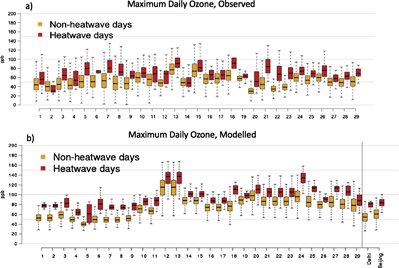
Figure 2. Box-and-whisker plots showing median (solid horizontal black line at center), 25th–75th percentiles as lower and upper boundaries of box, and 5th–95th percentiles as bottom and top whiskers for non-heat wave days (orange) compared to heat wave days (red) for surface ozone concentration (ppb) for (a) observations from 29 sites across the US (see map of locations in figure S2), and (b) same as (a) except with model values at the closest gridpoint, also including values for Delhi and Beijing at far right.
Download figure:
Standard image High-resolution imageNOx emissions from the fixed ozone precursor sensitivity experiment are also shown for each region in figure 1. A geographic depiction of the changes in prescribed NOx emissions for RCP6.0 and the stabilized ozone precursor experiment, where ozone precursor emissions are held fixed at 2005 levels, is shown in figure S1 available at stacks.iop.org/ERL/13/064004/mmedia for comparison with the regionally-averaged changes in figure 1.
3. Results
The CAM-chem model has a well-documented high bias of about 10–30 ppb for summer ozone concentrations (e.g. Val Martin et al 2015, Phalitnonkiat et al 2018), similar to biases in other Earth system models (Rieder et al 2015, Wu et al 2008, Rasmussen et al 2012, Parrish et al 2014). This high bias can be partly attributed to coarse resolution (e.g. 2 degrees in CAM-chem), which convolves urban and rural ozone concentrations and dilutes precursor emissions resulting in an overestimation of nighttime ozone in urban areas due to reduced titration (e.g. Pfister et al 2014). Though this high bias is a consistent feature of Earth system models, their responses to changes in forcing have been shown to be more comparable to observed responses, and thus remain useful as tools to study physical processes involved with changes in ozone precursors (e.g. Pfister et al 2014, Rieder et al 2015).
This high bias can be seen in scatter plots of summer maximum daily surface ozone concentration and maximum surface temperature at the 29 ozone observational sites in the US (see figure S2 for a map of site locations) compared to similar locations from the model simulation (figure S3). The linear fits to these scatterplots of observations have a variety of slopes ranging from near zero to about 4 ppb K−1. Comparable locations from the model in figure S3b (including two non-US sites, Delhi and Beijing) show slopes with a similar range, from near zero to about 5 ppb K−1. This is within the range of slopes reported in the literature, from near zero to about 6 ppb K−1 (Rasmussen et al 2012, Brown-Steiner et al 2015).
To assess the CAM-Chem simulation of surface ozone concentrations during heat waves, figure 2(a) shows box-and-whisker plots for the 29 sites in the US in figure S2. Surface ozone concentrations are shown for summer non-heat wave days as well as heat wave days. For 27 out of the 29 sites, median ozone concentrations increase during heat waves, with magnitudes ranging from about 10%–80%. Model-simulated values for those same locations are shown in figure 2(b). The previously noted high bias for summer ozone of about 30 ppb is evident, with non-heat wave day median values for observations ranging from about 40–80 ppb compared to model values of about 50–120 ppb. However, in terms of the simulated ozone concentrations during heat waves, all locations show an increase relative to non-heat-wave days (including the two non-US sites near Delhi and Beijing at far right) with median increases ranging from about 10%–60%, in roughly the same range as the observations.

Figure 3. Average maximum daily temperature (°C) during heatwaves for 1986–2005 (top row), changes for midcentury (2046–2065 minus 1986–2005, middle row) and end of the century (2080–2099 minus 1986–2005, bottom row). RCP6.0 (with varying ozone precursors) at left; simulations with anthropogenic ozone precursors fixed at 2005 values at right. Values are not plotted for areas poleward of 60 degrees North and South.
Download figure:
Standard image High-resolution imageFor additional context, future time periods in the 21st century show a decrease in the linear slope of the temperature-ozone relationship for the US sites in the RCP6.0 experiment (figure S4). This is consistent with previous results showing that the slope decreases as precursor emissions decrease (Rasmussen et al 2012). However, there is virtually no change in the slope from 1986–2005 to 2080–2099 for Delhi and only a small increase in the slope for Beijing, a reflection of the small changes to ozone precursor emissions in RCP6.0 at those locations over the 20th century. However, in 2046–2055 there is an increase of the slope at Beijing to a value over 5 ppb K−1, showing that over Asia, increasing heat wave intensity during mid-century is likely to increase ozone pollution events. Meanwhile, for the stabilized ozone precursor emission experiment, the slopes are more comparable between present and future time periods at all sites (figure S5) associated with the fixed ozone precursors. However, as noted above, Asia is different since NOx emissions are smaller in 2005 than for mid-century conditions. This will be discussed further below.
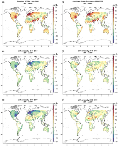
Figure 4. Difference in surface ozone concentration (ppb), heat wave days minus non-heat wave days, (a) 1986–2005 reference period; (b) same as (a); (c) RCP6.0, 2046–2065; (d) same as (c) except for stabilized ozone precursor experiment; (e) same as (c) except for 2080–2099; (f) same as (d) except for 2080–2099. Values are not plotted for areas poleward of 60 degrees North and South.
Download figure:
Standard image High-resolution image
As noted above, it has been established that as mean temperature increases, heat waves are projected to become more intense. This can be seen in figure 3, where the daily maximum temperatures during heat waves (Tmax) increase in all regions, with maximum values increasing up to 2° in central North America and parts of Europe for the last 20 years of the 21st century compared to 1986–2005 (figure 3(c)). Values of maximum surface temperature on heat wave days are greater than on non-heat wave days by about 2 °C–5 °C in most tropical and subtropical areas, and 7 °C–10 °C at higher latitudes (figure S6). These higher temperatures during heat wave days in the reference period of 1986–2005 produce increases of ozone concentration of about 2–10 ppb (roughly 10%) on heat wave days compared to non-heat wave days in most regions (figures 4(a) and (b)). Due to the prescribed changes of ozone precursors in RCP6.0 (e.g. Figure 1 and figure S1), maximum values of surface ozone during heat waves (left side of figure 4) are lower in future heat wave days compared to non-heat wave days, with negative differences of about −10 to over −20 ppb (about 10% to over 50%) over much of the US and Europe by mid-century (figure 4(c)), with additional decreases of up to 30–60 ppb (about 50%–100%) by late century. In contrast, small increases of roughly 10–30 ppb occur over parts of the Mideast, eastern Asia and northern Africa by mid-century, while over eastern Asia, with the decreases of ozone precursor emissions by late century (figure 1 and S1), there are decreases of ozone in heat wave days compared to non-heat wave days of about 5–10 ppb there (figure 4(e)).
Given that heat waves are more intense in the future warmer climate in the stabilized ozone precursor experiment, one could assume that ozone concentrations should be larger everywhere in future heat wave days compared to non-heat wave days in that experiment. But figures 4(d) and (f) show a regional pattern to the differences. There are increases of ozone on heat wave days compared to non-heat wave days (positive differences) over central and northeastern North America, western Europe, and most of central Asia by mid-century with differences of about +5 to +10 ppb (on the order of 10%). However, even with increases in maximum temperatures in heat waves (figures 3, S6), some regions experience decreases of ozone in heat wave days compared to non-heat wave days in a future warmer climate (e.g. west coast and southeastern North America, eastern Europe, and northeastern Asia).
The difference in regional responses of ozone in heat waves between RCP6.0 and the stabilized ozone precursor experiment depends on the details of the relationship between ozone concentration and maximum temperature. Linear fits for this relationship were shown in figures S3, S4 and S5. In figure S7 nonlinear fits are shown for the RCP6.0 experiment for two sites in the southeastern US (top panels), and two sites in the northeastern US (lower panels). For all four sites, the ozone concentrations on future heat wave days (pink dots, red line and symbols) are less than for present-day heat wave days (gray dots, black line and symbols) and produce negative differences as could be expected from figures 4(c) and (e). Additionally, the large negative differences in figure 4(e) for late century indicate that the decreases in ozone concentrations are proportionately larger on heat wave days compared to non-heat wave days in RCP6.0. The reason for this can be seen for all sites in figure S4 and for these four sites in figure S7 such that the slope for the future ozone-temperature relationship is flatter compared to the present-day slope. Because of this difference in slopes, the negative ozone concentration differences for heat wave days are on the order of twice as large as for non-heat wave days.
To understand the areas with the positive differences in the stabilized ozone precursor experiment, examples of two sites in the northeastern US are shown in the bottom panels of figure S8. The slopes of the present and future nonlinear fits are nearly the same, and the differences of ozone in future heat wave days minus present heat wave days are positive in both locations (on the order of 10%). Similarly, the differences of ozone on future non-heat wave days minus present non-heat wave days are positive in both locations (on the order of 10%). However, for the sites in the southeastern US (figure S8 top panels), the fits are more nonlinear, with a somewhat reduced slope of the ozone-temperature fit in the future compared to present. Therefore, the difference in ozone concentrations on future heat wave days minus present heat wave days is negative (about 10%–15%), while the ozone on future non-heat wave days minus present non-heat wave days is small positive in both locations (on the order of 10%). The reason for the reduced slope in the future compared to present in the southeastern US locations (and also in west coast North America) that produces the negative differences in those regions in figure 4(d) and (f) is associated with ozone suppression in those locations likely related to isoprene emissions that are a function of temperature (Wu et al 2008, Steiner et al 2010, Guenther et al 2006).
For further context, the time series of summer Tmax for four US and two Asian cities (Delhi and Beijing) show that the 21st century trend of summer Tmax is positive for both the RCP6.0 and stabilized ozone precursor experiments for all six cities (figure S8), while the time series of maximum daily summer ozone follows the time evolution of NOx (figure 1 and figure S1) with decreases in many locations. For example, for the US cities the values of maximum ozone start to decline in the late 20th century and continue to decrease through the 21st century in RCP6.0. Meanwhile, for Delhi and Beijing compared to the US cities, there are relatively lower concentrations of surface ozone at the end of the 20th century with small increases that continue until around mid-century and decrease thereafter. In the stabilized ozone precursor experiment, there is a small but steady increase in maximum surface ozone concentrations throughout the 21st century for all six cities, with similar increasing trends in Tmax.
4. Conclusions
Though CAM-chem has a high bias for simulated surface ozone concentrations, the model simulates a response to changes in present-day ozone precursors with increases of roughly 10%–80% in median surface ozone concentrations in heat wave days compared to non-heat wave days. These are comparable to increases of about 10%–60% for selected US sites with ozone observations that are evaluated in this paper. Due to the specification of reductions in ozone precursors based on the assumption of policy changes in RCP6.0, maximum surface ozone concentrations are projected to decline in North America and Europe during heat waves, even as heat waves become more intense. Meanwhile, in regions of Asia there are increases in surface ozone concentrations by mid-century during more intense heat waves in the future and increases in ozone precursors in RCP6.0.
To assess the changes that would result if assumed policy measures that reduce future ozone precursors did not materialize for the US and Europe, an alternative set of simulations is performed where anthropogenic ozone precursors are held constant at 2005 values and all other forcings follow RCP6.0. Future maximum temperatures in heat waves increase in both the RCP6.0 and the stabilized ozone precursor experiments. However, projected maximum ozone values in heat wave days compared to non-heat wave days increase with more intense future heat waves for most areas in the stabilized ozone precursor experiment (northeastern North America, western Europe, central and northern Asia), but decrease in others (e.g. coastal and southeastern North America, eastern Europe, northeastern Asia) pointing to the likely role of ozone suppression related to isoprene emissions in those area. Meanwhile, in RCP6.0 most areas show decreases in ozone concentrations in future heat wave days compared to non-heat wave days as the slope of the ozone-temperature relationship decreases in a future warmer climate with decreases of ozone precursor emissions.
This study identifies the relationship between ozone and temperature during heat waves globally and illustrates that temperature is not necessarily a primary control on modelled ozone concentrations in future heat waves. This is due to the dependence on how ozone precursors are prescribed in future emission scenarios, and how related emissions of VOCs can be affected by temperature and influence ozone concentrations. Because of these factors, heat waves in a future warmer climate cannot necessarily be associated with a particular air quality outcome. Reducing ozone precursor emissions will help to improve air quality, but will only have a small direct contribution to mitigation of climate change. However, reducing surface ozone concentrations may increase the capacity for vegetation to store carbon, and can therefore have an indirect effect on mitigation of climate change (Lombardozzi et al 2015, Sitch et al 2007).
Acknowledgments
The authors acknowledge Lu Shen for providing the observed ozone data, and Gary Strand for processing the model data. Portions of this study were supported by the Regional and Global Climate Modeling Program (RGCM) of the US Department of Energy's Office of Biological & Environmental Research (BER) Cooperative Agreement #DE-FC02-97ER62402, and the National Science Foundation. Computing resources (ark:/85065/d7wd3xhc) were provided by the Climate Simulation Laboratory at NCAR's Computational and Information Systems Laboratory, sponsored by the National Science Foundation and other agencies. The authors acknowledge the Aspen Global Change Institute (AGCI) and its director, John Katzenberger, for hosting a workshop in the summer of 2016 that laid the foundations for this paper, along with the attendees who contributed to discussions that led to the research described herein.