

Abstract
The Paris Agreement on climate change aims to limit 'global average temperature' rise to 'well below 2 °C' but reported temperature depends on choices about how to blend air and water temperature data, handle changes in sea ice and account for regions with missing data. Here we use CMIP5 climate model simulations to estimate how these choices affect reported warming and carbon budgets consistent with the Paris Agreement. By the 2090s, under a low-emissions scenario, modelled global near-surface air temperature rise is 15% higher (5%–95% range 6%–21%) than that estimated by an approach similar to the HadCRUT4 observational record. The difference reduces to 8% with global data coverage, or 4% with additional removal of a bias associated with changing sea-ice cover. Comparison of observational datasets with different data sources or infilling techniques supports our model results regarding incomplete coverage. From high-emission simulations, we find that a HadCRUT4 like definition means higher carbon budgets and later exceedance of temperature thresholds, relative to global near-surface air temperature. 2 °C warming is delayed by seven years on average, to 2048 (2035–2060), and CO2 emissions budget for a >50% chance of <2 °C warming increases by 67 GtC (246 GtCO2).
Export citation and abstract BibTeX RIS

Original content from this work may be used under the terms of the Creative Commons Attribution 3.0 licence.
Any further distribution of this work must maintain attribution to the author(s) and the title of the work, journal citation and DOI.
1. Introduction
Reflecting the 90%–100% consensus among relevant research [1, 2], the 5th Assessment Report of the Intergovernmental Panel on Climate Change (IPCC AR5) stated that 'warming of the climate system is unequivocal' and 'It is extremely [95%–100%] likely that human influence has been the dominant cause of the observed warming since the mid-20th century'. [3] Such scientific findings can inform policy responses in concert with other factors such as risk aversion, discounting of the future and assessments of the severity of future climate impacts. The Paris Agreement of the United Nations Framework Convention on Climate Change (UNFCCC) Article 2.1(a) expresses a long-term goal of:
'Holding the increase in the global average temperature to well below 2 °C above pre-industrial levels and pursuing efforts to limit the temperature increase to 1.5 °C above pre-industrial levels, recognizing that this would significantly reduce the risks and impact of climate change'.
However, 'global average temperature' is not precisely defined, and achievement of the Agreement's goal may depend on possible different definitions and available measurement techniques. A related concept is that of a carbon budget, the allowable cumulative carbon dioxide (CO2) emissions consistent with a specified level of peak warming with a particular probability [4–6].
The IPCC 5th Assessment Report (AR5) assessed carbon budgets for various levels of warming in billions of tonnes of carbon (GtC) or of carbon dioxide (GtCO2) based on projections of global near-surface air temperature change, which we refer to as 'global-tas', where tas means 'temperature, air, at surface', from complex Earth System Models (ESMs). In general, climate modelling studies use global-tas, whereas observational records typically combine non-global coverage of near-surface air temperature over land with sea-surface temperature (SST) over oceans. As it is likely that stakeholders may have diverse interpretations as to what global average temperature refers, here we provide carbon budgets for different definitions of global average temperature, including definitions consistent with current observational products. Three main factors contribute to differences in 'global average temperature' change between global-tas and observational records. Firstly, there are regions with missing data that may not warm at the global-mean rate. For example, the Arctic is now rapidly becoming warmer and wetter [7], but much of it is commonly excluded due to lack of long-term data [8]. Secondly, under CO2-driven global warming, modelled near-surface air temperatures warm more than SSTs [9]. Finally, data providers must decide how to account for changes in sea ice. There may be a change from reporting estimated near-surface air temperatures to SSTs where ice has retreated. In the HadCRUT4 dataset [10] this approach probably results in an artificially low reported warming compared with the air warming due to features of the normalisation procedure.
We refer to issues related to missing data as being due to 'masking', and the other two factors together as 'blending', specifically 'air-sea blending' and 'sea-ice blending'.
One early study accounted for the masking and air-sea blending issues [11], and some studies have accounted for masking but this is not universal. Recently, it was shown that over 1861–1880 to 2000–2009, modelled global-tas increased 24% more than a HadCRUT4 like blended-masked estimate [12]. Current observed temperature records should therefore exceed 2 °C later than global-tas, implying a larger carbon budget if compliance were assessed using one of them. Here we extend this prior work by (i) reporting results to 2099, (ii) calculating carbon budgets using IPCC techniques, (iii) accounting for realistic potential future data coverage and (iv) applying blending and masking to a low-emission scenario. In particular, the addition of a low-emission scenario allows us to determine to what extent temperature definitions matter if policymakers choose to take strong mitigation action.
Future blending-masking biases may change relative to the past because of increased modern data coverage: indeed, the blending-masking bias under transient warming with 2000–2009 data coverage was estimated to be 15% instead of 24% [12]. Furthermore, with strong mitigation sea-ice cover would be expected to stabilise before 2100, suppressing the future sea-ice blending bias [13]. In addition, the long-term warming pattern may differ from the historical pattern, leading to a different effect of coverage bias [14–16].
2. Methods
We consider two emission scenarios from the Coupled Model Intercomparison Project, phase 5 (CMIP5): the low emissions Representative Concentration Pathway 2.6 (RCP2.6 [17, 18]) and the high emissions RCP8.5 [19]. Among CMIP5 scenarios, only RCP2.6 has a substantial probability of <2 °C warming so we use it as representative of a world of strong mitigation. This allows us to estimate shifts in the probability of compliance with Paris targets in such a world, and to determine whether the magnitude of blending and masking biases should change substantially in the future. Meanwhile, RCP8.5 is used to estimate carbon budgets in a manner that is comparable with a set reported by the IPCC 5th Assessment Report. Note that we report decadal temperature changes relative to 1861–1880 to include simulations beginning in 1861 and avoid major volcanic eruptions. Supplementary figures 1 and 2 available at stacks.iop.org/ERL/13/054004/mmedia further justify the choice of these reference periods.
We process CMIP5 simulations on a 1 × 1° lat-lon grid using the Cowtan et al (2015) [20] algorithm and assuming that 2005–2014 geographic data coverage is maintained in future. This is done by downsampling the HadCRUT4 historical coverage up to December 2014 to 1 × 1° and extending this coverage to December 2099 in the following fashion. For each calendar month, coverage is allowed if data are reported at that location for that calendar month in more than 5 years from 2005–2014 inclusive. Mapping at 1 × 1° instead of 5 × 5° does not affect reported global temperature but keeps spatial information that may be useful in future. We area weight all reporting cells, whereas HadCRUT4 calculates hemispheres separately then averages those: this introduces a minor 1.9% difference in 1861–2016 warming (supplementary figure 3).
We calculate four temperature series for each simulation beginning with the widely used 'global-tas', and then add the effect of SST blending by mixing air temperatures and SSTs before calculating the anomalies, which we call 'air-sea blended'. Next, we add the effect of sea-ice blending by calculating the anomalies in air and ocean temperatures separately before combining them, and call this 'fully blended'. Finally we restrict coverage to follow the historical or assumed future HadCRUT4 like data availability and call this 'blended-masked'.
We select all CMIP5 simulations that have continuous historical and RCP2.6 or RCP8.5 runs from 1861–2099 inclusive and for which we could obtain the required output fields. These fields are Near-surface Air Temperature (short name 'tas'), Sea Surface Temperature (SST, 'tos'), Sea Ice Concentration ('sic') and Sea Area Fraction ('sftof', see the CMIP5 Standard Output description at http://cmip-pcmdi.llnl.gov/cmip5/data_description.html). Simulations are listed in supplementary tables 1 and 2 and model configurations can be found in table 9. Table 9.A.1 of AR5 [21]. Each simulation was processed using the Cowtan et al (2015) code and our updated future coverage mask. Blended temperature at the i,jth grid point, Tblend,i,j is obtained using:

where wair,i,j is the fraction of the grid cell from which near-surface air temperatures are taken, Tair,i,j refers to the local air temperature 'tas' and Tocean,i,j the local SST 'tos'. Each of these is converted into temperature anomaly relative to the local baseline of the same type (i.e. air or water). After the local anomalies are calculated, the grid points are then averaged with a spherical Earth area weighting. For global-tas, wair = 1 always, while for blended series wair,i,j is the fraction of land plus sea ice within the grid cell. For air-sea blended, a grid cell's wair,i,j is fixed based on the initial sea ice extent whereas for fully blended the sea-ice fraction changes depending on the monthly sea ice concentration.
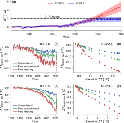
Figure 1. (a) CMIP5 global near-surface air temperature change under RCP2.6 and RCP8.5 relative to 1861–1880, with the ensemble median as a line and the shaded area representing the 5%–95% ensemble range (r1i1p1 simulations only). ((b) and (d)) The difference for each scenario (as labelled) between the CMIP5 ensemble median blended-masked temperature change and the global tas-only, shown as blended-masked minus tas-only. Each line represents one extra blending or masking factor: blue is ocean-blend only, green is ocean-blend plus sea-ice blend, and red is both blends plus masking for data coverage. On the right of the figure, each point and bar represents the ensemble median and 5%–95% range of each difference for the final decade. ((c) and (e)) decadal means of the differences from ((b) and (d)) plotted as a function of the global tas-only temperature change relative to 1861–1880 for the labelled scenario.
Download figure:
Standard image High-resolution imageCarbon threshold exceedance budgets (TEBs) are calculated as in the Technical Summary of IPCC AR5 [22]. Linear interpolation between decadal means are used to compute the diagnosed cumulative CO2 emissions since 1870 to the point that warming exceeds a given temperature threshold. Unlike in ref. [22], only complex ESMs are included in the analysis with Earth system models of intermediate complexity (EMICs) excluded. Reported percentiles correspond to percentiles of the distribution of ESM TEBs for that warming threshold. ESMs (models that can interactively diagnose compatible CO2 emissions with a prescribed concentration pathway) considered here are identified with an asterisk in supplementary table 2.
3. Results
3.1. Effect of temperature definition under low emissions.
Figure 1(a) shows the CMIP5 historical-RCP2.6 and historical-RCP8.5 ensemble time series of global-tas. Figure 1(b) shows the blending-masking differences and figure 1(c) the decadal averages of these differences as a function of global-tas for historical-RCP2.6 and panels (d) and (e) the same for historical-RCP8.5. All results shown here use a single simulation from each model, labelled 'r1i1p1' in CMIP5 nomenclature. Results are not sensitive to including the full ensemble (supplementary table 3 and supplementary figure 4).
In RCP2.6 the air-sea blending bias stabilises in the last ~70 years of the simulations while figure 1(c) shows that the sea-ice-blending and masking biases increase with global-tas throughout the series, but at a much slower rate than under RCP8.5. This suggests that the temperature stabilisation reduces sea-ice loss and its contribution to reported temperature bias. Similarly, the error bars in figure 1(b) show that uncertainty introduced by sea ice change is smaller under RCP2.6.
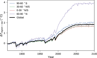
However, temperature bias still continues to grow with time in RCP2.6, and figure 2 demonstrates that the masking bias component is likely dominated by the warming at high northern latitudes, which tend to warm much more than the global average and are poorly sampled.
Figure 2. Time series of mean CMIP5 near-surface air temperature change from 1861–1880 under historical-RCP2.6 scenario split into latitude bands as labelled in the legend. The solid black line shows the global-tas value, undersampling of any region that shows warming above this black line will lead to a cooling masking bias, and vice versa. The modelled bias is dominated by undersampling of the northern high latitudes where by far the greatest warming occurs.
Download figure:
Standard image High-resolution image
Table 1 contains the ensemble median and 5%–95% range for RCP2.6 and RCP8.5 temperature changes over periods spanning the past (1861–1880), present (2007–2016) and future (2090–2099). Under RCP2.6, the percentage of simulations consistent with 2 °C warming increases from 75% for air-sea blended (the same as for global-tas) to 90% for blended-masked. Percentage blended-masked bias is calculated separately for each simulation and the median and ranges of these percentages are reported: the 16% bias for 1861–2016 differs from the 24% reported previously [12] due to the changed time period, available RCP2.6 runs, and because this result doesn't use the same HadCRUT4 hemisphere-weighting.
Table 1. Percentage increase in observed temperature change between selected periods when considering global-tas relative to the blended or blended-masked version. 'Fully blended' includes the sea-ice change effect in addition to air-water warming differences. CMIP5 ensemble median reported with 5%–95% range in brackets. Bottom row shows the number of simulations and percentage of ensemble that show <2 °C difference between 1861–1880 and 2090–2099.
| (ΔTglobal - tas - ΔTblended)/ΔTglobal - tas (%) | ||||||
|---|---|---|---|---|---|---|
| historical-RCP2.6 | historical-RCP8.5 | |||||
| Period: | Air-sea blended | Fully blended | Blended-masked | Air-sea blended | Fully blended | Blended-masked |
| 1861–1880 to 2007–2016 | 5.8 (3.2–7.3) | 8.7 (6.0–10.9) | 16.2 (5.2–28.7) | 5.8 (3.9–7.4) | 8.9 (6.2–11.7) | 17.9 (5.5–27.1) |
| 2007–2016 to 2090–2099 | 1.9 (0.5–3.9) | 6.9 (3.9–12.0) | 10.6 (1.2–29.7) | 4.0 (2.5–6.1) | 10.1 (8.4–11.7) | 11.7 (8.2–15.9) |
| 1861–1880 to 2090–2099 | 4.2 (2.3–6.3) | 8.0 (5.4–9.8) | 14.9 (5.7–20.6) | 4.3 (2.8–6.3) | 9.7 (7.3–11.4) | 12.8 (7.4–18.1) |
| Cases with ΔT < 2 °C | 15/20 (75%) | 15/20 (75%) | 18/20 (90%) | N/A | N/A | N/A |
The ensemble suggests a decrease in air-sea blending bias in future, with global-tas warming from 2007–2016 to 2090–2099 just 1.9% (0.5%–3.9%, all bracketed values 5%–95% ensemble range) greater than the air-sea blended value. In addition, improved geographical data coverage relative to most of the historical period reduces the masking bias, although the ice-blending issue remains at a similar magnitude. Overall, 21st century global-tas warming is 10.6% (1.2%–29.7%) greater than the blended-masked estimate. The full-period blending-masking bias from 1861–1880 is approximately 14.9% (5.7%–20.6%).
As masking contributes the most to our blending-masking biases we assess whether our model-based estimates are realistic by considering observational data records that handle land data in different ways and have different masking biases. These datasets are HadCRUT4 [10], Cowtan and Way [8] and Berkeley Earth, [23, 24] all of which combine land air temperature data with the HadSST3 ocean product [25, 26] and extend over our full period. HadCRUT4 is subject to the full blending-masking bias while Cowtan & Way follows the HadCRUT4 method except that missing regions are infilled by kriging, a statistical method that accounts for spatial covariance in the field and more heavily weights nearby data. Berkeley Earth uses a similar approach, but handles the raw station data in a different manner.
From 1861–1880 to 2007–2016 the global warming in HadCRUT4 is 0.84 °C, in Cowtan & Way is 0.94 °C and in Berkeley Earth is 0.99 °C. The two records which do not assume that regions of missing data warm at the global-average rate show 12%–18% more warming, the same order of magnitude as the masking biases inferred from CMIP5 simulations, although particularly poor historical coverage over the Antarctic and Southern Ocean means that infilling from neighbouring regions may be inadequate.
3.2. Carbon budgets and temperature thresholds under higher emissions.
IPCC AR5 carbon budgets correspond to cumulative emissions compatible with thresholds of modelled global-tas warming. Carbon budgets for a 1.5 °C or 2 °C warming in any form of blended or blended-masked estimate will therefore be higher than the corresponding IPCC AR5 budget. Budgets given in table 2 correspond to cumulative CO2 emissions since 1870 until the point of exceeding 1.5 °C or 2 °C warming (a threshold exceedance budget or TEB [22, 27]) under RCP8.5 (see Methods). The IPCC AR5 results are also included for comparison, and differ somewhat since they include EMIC runs and were reported to the nearest 50 GtCO2, or approximately 13.6 GtC.
For the blended-masked timeseries the 1.5 °C and 2 °C thresholds are reached a median 7–8 years later than for global-tas under this high-emission scenario. This has implications for carbon budgets, with the TEB for which 50% of the ESMs have warming below 1.5 °C increasing by 53 GtC (194 GtCO2) and 67 GtC (246 GtCO2) for the 2 °C threshold.
The IPCC carbon budgets were reported relative to 1870, but policymakers require up-to-date guidance to inform discussions related to the Paris Agreement. We therefore also calculate the remaining post-2015 carbon budget based on the ESM ensemble after adjusting for observed warming through 2015 following the approach of Millar et al (2017, [28]). For example, given that HadCRUT4 shows approximately 0.9 °C human-induced warming to 2015, another 0.6 °C results in a total of 1.5 °C. In our ESM simulations, the remaining blended-masked carbon budget with a >66% chance of <0.6 °C warming post-2015 is 246 GtC. However, if Berkeley Earth were to be used, then historical human-induced warming is greater. It would also likely show greater future warming for a given quantity of CO2 emissions too as Berkeley better approximates air-sea blended temperatures rather than the blended-masked approach of HadCRUT4. We estimate the remaining 1.5 °C budget at near 161 GtC in that case (see supplementary table 4 and related discussion).
4. Discussion
Here we have shown that achievement of the Paris Agreement's long-term goals could depend on the definition of 'global average temperature'. The scientific background to the Paris Agreement was informed directly by the Structured Expert Dialogue [29], which used blended datasets with a wide range of coverage to track warming to date. Our results indicate the potential impact of choosing different types of observational product in the future to measure global temperatures in the context of the Agreement. As it is unlikely that estimates of global mean air temperature, which inherently rely on climate models, will be used, we show how the use of 'blended' observational products would increase the policy-relevant carbon budgets for 2 °C relative to the global air-temperature budgets given by IPCC-AR5 (see table 2).
Table 2. Estimated carbon budgets expressed in GtC for various percentiles of the ESM distribution for 1.5 °C or 2 °C global warming thresholds and different definitions of 'global average temperature'. The median and 5%–95% ensemble range of exceedance years are also shown and correspond to the full set of RCP8.5 CMIP5 simulations and not just the ESM subset.
| 1.5 °C budget (GtC) | 2 °C budget (GtC) | Year ΔT exceeded | ||||||
|---|---|---|---|---|---|---|---|---|
| Percentile of ESM distribution | >33% | >50% | >66% | >33% | >50% | >66% | 1.5 °C | 2 °C |
| IPCC since 1870 | 695 | 614 | 614 | 900 | 818 | 791 | — | — |
| global-tas | 703 | 667 | 588 | 931 | 852 | 794 | 2027 (2015–2039) | 2041 (2028–2053) |
| air-sea blended | 731 | 692 | 627 | 951 | 889 | 831 | 2030 (2018–2041) | 2043 (2031–2056) |
| fully-blended | 749 | 708 | 645 | 987 | 916 | 849 | 2031 (2018–2041) | 2044 (2032–2058) |
| blended-masked | 787 | 720 | 638 | 1053 | 919 | 855 | 2035 (2022–2044) | 2048 (2035–2060) |
A recent study estimated the post-2015 carbon budget with a >66% chance of achieving a 1.5 °C target at 204 GtC, rather than the 70 GtC implied by IPCC AR5, suggesting that the 1.5 °C target is 'not yet a geophysical impossibility', but likely requires 'strengthened pledges for 2030 followed by challengingly deep and rapid mitigation', i.e. cuts in net anthropogenic emissions (Millar et al 2017, [28]). The Millar et al value differs from IPCC-AR5 budgets as it updated these calculations using observed warming and emissions from a 2010–2019 reference period using CMIP5 consistent relationships between future warming and future CO2 emissions. A fraction of this difference was due to the IPCC carbon budgets being calculated for global-tas, whereas Millar et al used human-induced warming estimated from the blended-masked HadCRUT4 dataset, which would be approximately consistent with the '...observed impacts of climate change at 0.85 °C of warming' mentioned in the Structured Expert Dialogue, to define the remaining warming between the present-decade and 1.5 °C.
If an alternative observational dataset were used to monitor global temperature in the context of the Paris Agreement then estimates of human-induced warming and compatible carbon budgets would change. For example, the Berkeley Earth product uses infilling techniques with more data sources and a different sea-ice algorithm which should reduce differences with global-tas. It shows almost 20% more human-induced warming than HadCRUT4 through 2015, and hence would reduce post-2015 carbon budgets by around 80 GtC.
Biases associated with incomplete data coverage and the blending of air and water data both suppress reported warming relative to global near-surface air temperatures. Our analysis and results in table 1 indicate that these biases will tend to be smaller in future provided that the improved data coverage of recent decades is maintained. Furthermore, under a scenario of strong mitigation, the differences introduced by the retreat of sea-ice are smaller than under high emissions where sea ice retreat is more pronounced.
5. Conclusion
We have demonstrated here the importance of a clear understanding of different definitions of global mean temperature with regards to carbon budgets and achievement of long-term climate goals under the Paris Agreement. We propose that the definition of global mean temperature should be physically based, transparent and verifiable in order for stakeholders to have confidence in its value. For a timeseries to be truly 'global', it must account for the incomplete spatial coverage of direct observations, requiring techniques such as those used in Cowtan & Way or Berkeley Earth. It is key that policy-makers unambiguously elucidate how they intend to measure global temperatures in the context of the Paris Agreement to enable the most useful mitigation advice to be provide by the scientific community. If pure observation-based timeseries are used then further efforts for data-recovery in data-sparse regions would help, as would more long-term stations at high latitudes. In addition, the sea-ice blending effect is a non-physical artefact of algorithm design and it should be possible to account for this in future datasets. However, the long-term air-sea blending effect is difficult to verify due to the lack of robust, homogenised and long-term collocated air-SST ocean data, and its lack of measurability may justify the definition of global-average temperature as being an air-sea blended value. Under this definition, potential blending biases are reduced to an equivalent of an apparent 2–3 year delay in exceeding temperature targets, instead of the 7–8 years for a fully blended-masked series.
Acknowledgments
MR's contribution was carried out at the Jet Propulsion Laboratory, California Institute of Technology under contract with the National Aeronautics and Space Administration. RJM was financially supported by the Oxford Martin Net Zero Carbon Investment Initiative.