

Abstract
Individual-based models (IBMs) of complex systems emerged in the 1960s and early 1970s, across diverse disciplines from astronomy to zoology. Ecological IBMs arose with seemingly independent origins out of the tradition of understanding the ecosystems dynamics of ecosystems from a 'bottom-up' accounting of the interactions of the parts. Individual trees are principal among the parts of forests. Because these models are computationally demanding, they have prospered as the power of digital computers has increased exponentially over the decades following the 1970s.
This review will focus on a class of forest IBMs called gap models. Gap models simulate the changes in forests by simulating the birth, growth and death of each individual tree on a small plot of land. The summation of these plots comprise a forest (or set of sample plots on a forested landscape or region). Other, more aggregated forest IBMs have been used in global applications including cohort-based models, ecosystem demography models, etc. Gap models have been used to provide the parameters for these bulk models. Currently, gap models have grown from local-scale to continental-scale and even global-scale applications to assess the potential consequences of climate change on natural forests. Modifications to the models have enabled simulation of disturbances including fire, insect outbreak and harvest.
Our objective in this review is to provide the reader with an overview of the history, motivation and applications, including theoretical applications, of these models. In a time of concern over global changes, gap models are essential tools to understand forest responses to climate change, modified disturbance regimes and other change agents. Development of forest surveys to provide the starting points for simulations and better estimates of the behavior of the diversity of tree species in response to the environment are continuing needs for improvement for these and other IBMs.
Export citation and abstract BibTeX RIS

Original content from this work may be used under the terms of the Creative Commons Attribution 3.0 licence.
Any further distribution of this work must maintain attribution to the author(s) and the title of the work, journal citation and DOI.
Introduction
We will cover the history and current applications associated with individual-based models (IBMs), particularly gap models (Shugart and West 1980), used in forestry and forest ecology. The central concepts of these models are as old as forestry itself, although their application to the ecology and dynamics of mixed-aged and mixed-species forests require the computational power of modern digital computers. Their current applications can generate the expected stand structure and composition of forests starting either from bare ground or from a set of sample plots. Stand structure and composition are the summary of the births, deaths and growth of hundreds of trees on a collection of small plots. The models produce output that resembles raw field data and this has allowed development of multiple types of data-comparing model tests (see: Shugart 1984, Bugmann 2001, Shugart and Woodward 2011, Larocque et al 2016).
Agent-based models originated at about the same time in multiple fields,—astronomy, physics, forest ecology and several of the engineering sciences (Huston et al 1988). Many of these models were designed to solve 'middle-number' problems. These are problems in which the size and complexity among interacting objects are great enough to preclude simple solutions. The interactions in middle-number systems are sufficiently non-random and there is enough aggregate behavior to eliminate statistical-mechanical approaches (Kay 2008). This simultaneity was stimulated by the development of digital computers with much increased capacity to numerically solve middle-number problems. Arising from deep historical roots, challenging middle-number problems emerged in forestry about 60 years ago that involved the need to predict forest change under altered conditions (improved tree genetics, new environments, forest fertilization, tree spacing for non-native trees in plantations).
Hans Carl von Carlowitz's Sylvicultura Oeconomica (published in 1713) initially introduced the concept of 'scientific forestry' and sustainability (Nachhaltigkeit) to inform the management of forest lands intended to provide a sustainable supply of mining timbers to Silver mines in Saxony. In scientific forestry, the growth of single tree is based on determining the factors for the growth of a single tree (the Normalbaum or 'standard tree') in a particular environment. Empirical observations of thinning and growth of a large collection of standard trees in forest stands could analyzed as a 'large number' to be solved by statistical analysis for thinning rates to obtain the forest yield. This formulation is essentially an individual-based model of the relationship between the growth of an individual tree and the yield of a forest stand of such tree and growth-and-yield modeling remains central to quantitative forestry to the present. This up-scaling from the growth of a standard tree used and still uses empirical forestry 'yield tables', the bulwark of prediction for foresters. Today, when one drives into a university that has a forestry school or a forest research station, one often drives past 'experimental forests' of locally important, commercial tree species planted at different densities—the basis for calibrating regional forest-yield tables.
In the middle 1950s and 1960s, traditional forestry applications based on yield tables were challenged by several questions:
- How does one adjust yield tables to account for changes in growth from genetically-improved faster-growing trees?
- How can one develop yield tables for forests for which there are no empirical experimental data? This problem arose when trying to determine the appropriate densities and expected harvest schedules for the new forests including also new species combinations.
- Similarly, how does one derive a yield table for an introduced tree species, such as Pinus radiata, which was introduced as an exotic, softwood-timber-producing species in over forty nations?
- If one fertilizes a forest for improved growth of trees, how could yield tables be adapted to such situations?
- Particularly in the USA, how does one alter yield tables for the production of lumber that is measured in metric and not English dimensions?
An additional modern challenge is, 'how does one adjust yield tables for climate change?' These questions created a need for an answer, which involved discovering a rigorous procedure for the revision of standard yield tables.
Plantation forest models
One collection of approaches to developing a scientific basis for recalibrating yield tables was statistical. This focused on regularly spaced plantations of trees of the same species and age. Clutter (1963), Clutter et al (1983) parsed this problem into one of statistically deriving the parameters of two coupled derivatives: one for the change in the natural lobvolume of wood in a forest stand over the age of the stand (dlnV/dA) and a second for the change in basal area (the sum of the cross-sectional area of all the trees at a reference height) with age (dB/dA). Helpfully, if trees in the stand are all the same size, the basal area of the stand is simply the basal area of each tree times the density of trees, essentially the Normalbaum concept of Carlowitz. Empirical relations amongst tree height, the volume of a tree as a function of its diameter, changes in the increment of diameter as functions of tree density, or the local site conditions promoting tree growth to differing degrees make this a daunting mathematical estimation problem. This approach has the capability of ingesting records of forest plantation performance to obtain forest yield tables and to change these tables with changes in the growth rates of individual trees. It and its subsequent improvements are standard tools for plantation forestry (Burkhart and Sprinz 1984, Burkhart 1990). Embedded in these models are assumptions that all the trees in a stand are identical and that the stand density is fixed. These assumptions are appropriate for plantations but not so much for trees growing under more natural conditions.
Japanese forest ecologists tackled same problem of understanding patterns in the growth in diameters of trees in even-aged forest stands and the resultant change in stand volume (or biomass). Yoda et al (1963) developed a 'thinning law' to predict mortality in growing even-aged forests. Shinozaki et al (1964) produced the 'pipe model' concept that implied the sapwood cross-sectional area per unit of land provided a limit to growth and yield by relating the distributions of sizes and numbers of trees. Suzuki and Umemura (1974) visualized the prediction of growth and yield as a matter of understanding the change in the average size of a tree (tree growth) and the changes of the numerical distribution around the average tree for stands in which the trees were competing and eliminating weaker competitors (thinning). As smaller trees were overtopped and suppressed by the dominant canopy trees, the shape of the numbers distribution around the average tree changed in skewness and kurtosis around the average tree size change as a function of the population processes.
This Japanese-approach was applied to simulate the change in the distribution of tree sizes for the cohorts of trees in the gap left from the death of a large tree in temperate rainforests on Yakushima Island in southern Japan (Kohyama 1992) and subsequently to tropical rainforests in Borneo (Kohyama 1993). This latter approach was subsequently used as the computational engine for the ecosystem demography or ED model (Moorcroft et al 2001), which has been applied as a regional or global model for better understanding the dynamical role of forests in the global carbon cycle. This will be discussed below as a method to scale-up gap-model dynamics.
Mixed-aged and mixed-species methods
Kohyama's (1992, 1993) models represent a transition from the plantation modeling of growth and yield to the approximation of dynamics of forest mosaics. In general, yield tables have not worked well in forests comprised of trees of different ages (or sizes) or of different species. The problem of predicting change over time and managing for such forests generated an alternate approach to forest modeling that emphasized the growth and interaction of each individual tree in a simulated forest stand. The Normalbaum concept at the dawn of scientific forestry can be interpreted as an individual-tree-based modeling approach, and these new models were explicitly based on individual trees.
The first such model (Newnham 1964) was developed for Douglas-fir (Pseudotsuga menziesii) forests and predicted tree growth and stand yield for forest in which trees had non-regular spacing and were of different sizes. The subsequent development of similar models, developed in the doctoral dissertations at several Schools of Forestry, are archived in Forest Science, which at that time published the abstracts of forestry doctoral dissertations. These early forest IBMs were complex and large for the computers that were then being used to solve them.
For example, the competition among individual trees was typically simulated by crown interactions involving the three-dimensional geometry of each individual tree crown for all the trees in a stand (Newnham 1964); the growth of the tree trunks of each tree were often simulated at multiple heights (Hegyi 1974); tree mortality was related to two- or three-dimensional crown pruning among trees (Mitchell 1969, 1975). The most detailed early model, FOREST (Ek and Monserud 1974), also considered multiple tree species. In FOREST, tree competition derived from the interactions among the three-dimensional crown geometries (different idealized-shaped canopies were used for different species). FOREST mapped the exact locations of trees, calculated the dispersion pattern of seed-fall based on seed morphology, etc. It exceeds the complexity of virtually all modern forest IBMs.
This history of development of forest landscape models and their origins starting with forestry growth and yield models to more models operating at the landscape scales has recently been reviewed by Shifley et al (2017). They and we see the increased mechanistic complexity and physical dimension represented in spatial forest-landscape models developing over time as a consequence of the increase in computational power over the past decades. The effect arises can be related to the so-called Moore's Law, that the number of components in integrated circuits doubles about every two years (Moore 1965). In the case of landscape models, this increase in computational capability, has allowed the fusion of increasingly larger data sets into the models. Much of the functional complexity was found even in very early forest IBMs.
Gap models
In 1972, Botkin et al 1972 produced an important simplification of the earlier forestry work using IBMs, which they called the JABOWA model for the initials of its developers. A model (Siccama et al 1969) presented at the annual meeting of the Ecological Society of America has been cited as an earlier version of this model but based on its short description, it seems to be a different, more statistical approach. From a forest inventory plot, JABOWA annually computed diameter increment of each tree, it stochastically killed trees and planted new trees. Botkin et al (1972) did not cite any of the antecedent forestry models. Because the forestry IBMs were mostly, but certainly not entirely, in sources not frequently read by forest ecologists, the earlier forestry work remained sub rosa to most ecologists. Additionally, some of the forestry IBMs drifted into the realm of 'industrial secrets' as their developers found employment in the timber industry.
In 1980, Shugart and West introduced the term 'gap model,' to describe this class of models. The gap model designation emphasized that a principal simplifying assumption in these models (the assumption that the competition among individual trees on a small patch of land was homogeneous in the horizontal dimension across a small area but spatially explicit in the vertical dimension) related to the classic 'gap dynamics' concept of A.S. Watt (1925, 1947). Implied in this formulation was an underlying idea that a small plot, near the size of the influence zone of a large tree was an appropriate scale to include the gap generation and recovery seen in Watt's classic work. In practice, the plot size used in these models has been around 0.04 to 0.10 hectares depending on sizes and heights of trees. Gap models formulated at larger or smaller spatial scales can demonstrate dynamic responses that are anomalous to those of Watt's basic 'pattern-and-process' concept for forests (Shugart and West 1979). The ratio of height of a gap to its width changes the direct-light illumination zone of the forest floor as a function of latitude (Kuuluvainen 1992). In agreement with Kuuluvainen, the spatial unit used in gap models for models from the tropics to temperate to boreal zones have smaller plot sizes towards the equator matching the higher average sun angles there.
A generation of forest ecologists have made numerous extensions of 'gap models' and the term, nowadays, refers to a broad class of IBMs for forests and other ecosystems of a 'natural' character (mixed-age, mixed-species, natural disturbance regimes, etc). Modeling forest growth has been reviewed several times and it is our intention to recognize but not rehash this well-done work. Liu and Ashton (1995) reviewed gap models and tabulated the phylogeny of about 20 of these models springing from the JABOWA and FORET models. Porté and Bartelink (2002) used a hierarchical search algorithm to the papers in several abstracting data sets and found about 700 papers involving modeling mixed-forest stands published up to 2000. They produced a thoughtful review of the common issues of successes and needs across 199 of these models, including many gap models. Bugmann (2001) review presented and investigated details of model assumptions and formulations. Xi et al (2009) reviewed forest landscape models and placed gap models in the context of 'other, landscape-level simulators of forest dynamics'. Shugart and Woodward (2011) reviewed a large set of gap models and tabulated the testing of these against a wide range of forest data at different time and space scales. More recently, Larocque et al (2016) reviewed forest succession models, which simulate the long-term dynamic change of mixed-age, mixed-species forests and tabulated the significant functions and applications of each.
We searched the Web of Science for citations to 12 different early gap models (or model series) that each had more than one hundred citations since their publication. The three books in this collection were searched on Google Scholar and were also included in this analysis as is indicated in the legend of figure 1. Citations to these models show two strong peaks, one in the interval 1995–1996 and a second stronger peak in 1999–2001 (figure 1). The total number of publications that cite these articles totaled 6500 (up until the end of the year 2016). Some of these models show substantial 'longevity' and are still being cited regularly 30+ years after their initial publications. One would expect a transition to more recent papers, perhaps with revisions in the models, in the citation pattern over time. The decline in citations after 2001 in figure 1 appears to arise from the substitution citation of new versions of the original models or of more recently derived second-generation models derived from these early 12 gap models. Model developers of almost any ecological model tend to differentiate their creations from those developed by others.

Figure 1. Citations to early gap models from the Web of Science® and in the case of the two books from Google Scholar®. Searches were conducted on June 30, 2017 using the 'All databases' option in Web of Science. The searches were from the initial paper(s) that documenting for each model: JABOWA (Botkin et al 1972, Botkin 1993); FORET (Shugart and West 1977, Shugart 1984); FORTNITE (Aber et al 1978); LINKAGES (Pastor and Post 1986); ZELIG (Urban et al 1991); TreeDyn+ refers to the complex of functional-type based models (Bossel 1996) including the FORMIX-series of models (Huth et al 1998, Huth and Ditzer 2000); FORCLIM (Bugmann 1996); SORTIE (Pacala et al 1996); FORMIND (Köhler and Huth 1998, 2000); FORENA (Solomon 1986); HYBRID (Friend et al 1993).
Download figure:
Standard image High-resolution imageCurrently, there are hundreds of gap models in use for a wide array of local-to-regional applications. This is potentially confusing for non-model-oriented scientists trying to read across this literature. These models have more in common than many suspect. These gap models endorse the fundamental premise that the structure of forests promotes a remarkable control of ecosystem dynamics that is lost in more aggregated modelling approaches. This class of models has a surprising capability to predict responses of real forests over longer-than-annual time scales. Exercising the models has also produced useful theory on how forests could be expected to respond to change and what factors determine these patterns of change.
The issue of model complexity invariably arises in the development of forest IBMs. In general, an increase in model 'complexity' including number of parameters in a model, the amount of data needed to initialize the models, or the additional to functional couplings in a model has increased with computation power. Multi-level models, such as gap models with individual plant → plot → landscape → region → continent scaling are relatively simple when seen across one of the levels, but are complex when seen through multiple levels. Most ecological modelers realize that there is a trade-off between model simplicity and model complexity that results in a 'sweet-spot', the so-called Medawar zone (see: Medawar 1967, Grimm et al 2005). Differences in objectives in a given study preclude the universal acceptance of any one model approach as always being the most appropriate choice, even when restricted to the case of individual-based models simulating forests.
General functioning of gap models
Gap models intentionally feature relatively simple protocols for estimating the model parameters (Shugart 1984, Shugart and Woodward 2011). For many of the more common temperate and boreal forest trees, there is a considerable body of information on the performance of individual trees (growth rates, establishment requirements and height/diameter relations) that can be used directly in estimating the parameters of such models. Parameter estimation is aided by many of the parameters in the model being tangible attributes of tree species: their maximum growth rate, their maximum heights, their tolerance of shading, drought, nutrient stress, etc.
One obvious approach to simplifying this class of models would be to represent the species in the models with some reduced number of 'functional types' of plants. Since the computation burden in the models stems from the processing of individual trees, the main advantage is in the reduction of the demands for parameter estimation for each species of tree considered. Hartmut Bossel and colleagues (Bossel 1991–1996, Bossel and Krieger 1991–1994, Köhler et al 2000, Huth and Ditzer 2000–2001) pioneered this approach for tropical rain forests. Such models have subsequently found wide applications in Borneo, French Guiana and in several other tropical ecosystems, as well as for forest at the global scale. Two examples will be discussed in more detail in the sections below for the FORMIND model (Fischer et al 2016, Köhler and Huth 1998) and the FORCCHN (Ma et al 2017) model.
Gap models have simple rules for interactions among individuals (e.g. shading, competition for limiting resources, etc) and equally simple rules for birth, death and growth of individuals. The simplicity of the functional relations in the models has positive and negative consequences. The positive aspects are largely involved in the ease of estimating model parameters for a large number of species; the negative aspects with a desire for more physiologically or empirically 'correct' functions. An earlier synthesis (Shugart 1984) was entitled 'A Theory of Forest Dynamics' with the 'A' intended to emphasize that the theoretical implications of these models are necessarily special theories—the theoretical implications and practical applications are constrained by the underlying gap-model assumptions.
To elucidate some of these assumptions, figure 2 outlines the general features in gap models. The essential modelling functions of a gap model resemble those of other IBMs for forests. In most gap models, the diameter of each tree is updated annually and the parameters of the diameter growth equation vary with species. The original JABOWA and FORET models incremented volume of wood and used allometric equations derived from species' maximum heights and diameters to include a species' geometry in the diameter increment equation. Others have used other methods of incorporating tree geometry in the parameterization. For examples, FORSKA (Leemans and Prentice 1987, 1989) and FAREAST (Yan and Shugart 2005) models used a diameter-increment equation based on a pipe-model approach (Shinozaki et al 1964). OVALIS (Harrison and Shugart 1990) simulated tree form with both the heights and diameters dynamically changing in the model. Larocque et al (2016) provides a summary of these and other functions used across a large set of gap models and should be consulted for those interested in more details on these functions and the relationships that are discussed here and immediately below. They present a six-page table summarizing the internal functions for tree growth, competition, etc in 23 gap models as well as the trade-offs in the use of the different functions.
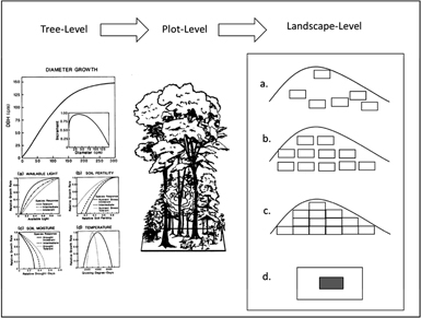
Figure 2. General functioning of a gap model. As one moves to the right to left, spatial scale increases from an individual tree to a small plot to a landscape. The tree-level response shown here is the elementary growth (or tree ring) equation from the FORET (Shugart and West 1977) model. The magnitude ot the tree-mortality probablity of each tree are also determined at the tree-level depending on tree growth as an index of vigor, species longevieties and other conditions. The form of the growth equation with no constraints is shown at the top and the decrement to this optimal growth equation is found below according to the particular controlling environmental factors (available light, soil moisture, etc). At the plot level, the vertical profile of light, available soil moisture, and other environmental and biogeochemical factors are calculated and tree to tree interactions are computed. Conditions for potential new seedlings for each year are determined factors such as the environmental conditions and seed sources. At the landscape model, a basic gap model can be used to represent the landscape as: (a) the summation of a Monte Carlo collection of independent random points; (b) gridded points at some spacing, (c) a tessellation of adjacent plots; (d) a spatially explicit landscape simulation with a spatial map of trees that is 'windowed' or updated for tree birth, growth and death by dropping a gap-model computational window onto the tree-stem map to solve for a subset of a new map. This is repeated to produce the new map. The size of this subset determines the resolution of the spatial map.
Download figure:
Standard image High-resolution imageThe species' growth equations (one equation per tree) invariably contain individual tree size as one important variable and are implemented as a differential or difference equations. The coupling of these equations is based on decreased individual growth in response of species specific responses to environmental factors (the vertical light profile, the nutrient availability for the plot, soil moisture, etc, see figure 2). These factors are computed at the plot level and require the implementation of biogeochemical models for nutrient elements, hydrological models of evapotranspiration, light extinction as a function of overhead light, etc.). The interaction among trees are a consequence of each tree's effect on the plot environment and the feedback of these environmental changes on each tree. Some gap models (e.g. FORMIND, FORCCHN) explicitly calculate each tree's biomass growth determined on the basis of a carbon balance including photosynthesis and respiration. Carbon-balanced-based tree growth is implicit in the formulation of most gap models. Mortality and establishment are also consequences of the mutually-modified and mutually-shared environment of the simulated plot.
In developing IBMs, one would like to avoid n-body problems, in which each individual interacts with each other individual, because the number of interactions then varies as a function of n2. For example, determining the shading of each tree on every other tree for hundreds of trees on a plot demands much, much more computation than simply computing the vertical profile of photosynthetically active radiation and then registering each tree against the computed light profile, as is done in most gap models. When spatially deriving the interactions of trees on a large landscape, n in the n-body problem becomes enormous, outstripping the capabilities of modern computers. Gap models are based on the assumption that the interactions among neighbours near the scale of a canopy gap are the dominant interactions (Watt 1947).
When averaged, the standard protocol for Monte Carlo simulation with stochastic models, gap models basically simulate landscape dynamics. In the simplest case (figure 2(a)), one simulates a large number of plots, which can be initialized by the species and diameters of each tree on sample plots with a matching spatial scale. As is the case in typical survey design, these plots are independent of one another (although they may share the same annual weather conditions, and perhaps large-scale disturbance events). The expected average of the landscape is the average of these simulated plots over time.
Because gap models are stochastic, comparisons between a single simulated plot to an actual re-measured sample plot are generally neither fruitful nor useful. After initialization with actual tree sizes and species from an actual forest sample plot, random events in the simulated plot, such as the death of a very large tree for example, would not be expected to occur in coordination those on the actual plot. An actual long-term reconstruction of plot-level field data would require a remarkably deep and detailed history of the sample plot. By analogy, a stochastic model of a pair of dice could predict the average proportions of numbers thrown over time. Indeed, it could be used to determine that real dice are 'loaded', but one would not expect the model to predict the next throw of the dice.
Perhaps for this reason, gap-model developers have generally had an interest in testing their models at the landscape- and larger-scale data. Shugart and Woodward (2011), chapter 5, provide numerous examples of such tests including:
- With a priori parameter estimation for species, predict forest-level features (total biomass, leaf area, stem density, average tree diameter, etc).
- Run model for a long period of time, predict mature forests preserved in a region.
- Calibrate model on stands of a given age, predict structure on stands of a different age(s).
- Use introduction of disease or change in conditions (e.g. fire frequency, droughts, disease such as the Chestnut Blight (Cryphonectria parasitica, etc) as 'natural' experiments.
- Predict independent tree diameter increment data, forestry yield tables, forest composition change along single environmental gradients, and forest composition response to multiple environmental gradients.
These tests of the models in cases involving gradient responses simulations are performed by placing clusters of simulation runs at grid locations across a landscape (figure 2(b)). Examples include tests against mountain altitudinal gradients (Kercher and Axelrod 1984, Bugmann 1996, Bugmann and Solomon 2000, Gutiérrez et al 2016, Yan and Shugart 2005, Foster et al 2017)
In more spatial applications, one can simulate a landscape as a tessellation with the land surface covered with adjacent plots of land. Applications have included dispersal of seeds from one cell to another or the spread of wildfire or other disturbances across the landscape (figure 2(c)). Finally, the ZELIG model (Urban et al 1991) simulates stem maps of tree (size and species) across a landscape map. The model is implemented by computationally 'dropping' a gap model on a small overlapping subsections of a stem map and then using the gap model to update the map. This is repeated to produce the next year's stem map, etc. The spatial resolution of the stem map spring from the overlap of the subsections. This computational procedure is called 'windowing' (figure 2(d)) and is a common general implementation for IBMs largely to reduce computational inefficiencies of spatially explicit models.
The ZELIG approach has been implemented in time plus three spatial dimensions and tested on its ability to reproduce fine-scale patterns in the autocorrelation structure of Douglas fir forests as measured by high-spatial resolution remote sensing (Weishampel et al 1992). More recently, Brazhnik and Shugart (2016) used a gap model with explicit spatial representation of the positions of the individual trees account for the effects of the flatter angles of direct light at high latitudes. This simulation includes the spatial effects of topographic shading (tall mountains to the south shading an area, the shadiness of steep valleys, etc) as well as the significant differences in north- and south-facing slopes along altitudinal gradients. Foster et al (2017) presents a similar investigation forest composition change with slope and aspect patterns as a gap model test in the USA Rocky Mountains. Spatial effects such as wildfire have also been represented in spatial forest IBMs (Brazhnik et al 2017).
Gap models can also be used to investigate questions related to biodiversity. In a case study, a gap model simulated the forest dynamics of a tropical rainforest with more than 400 tree species (Köhler and Huth 2004). It was shown that recruitment limitation and disturbance intensity are important for maintaining species richness (Köhler and Huth 2004). Besides species richness, forest management can play an important role for the development of forests. Logging has been included in forest gap models, allowing to simulate different logging strategies and to explore their long-term impacts on forest dynamics (Kammesheidt et al 2001, Köhler and Huth 2004).
It was shown that long logging cycles >60 years in combination with reduced-impact logging strategies could significantly reduce the negative long-term impact of logging on forest carbon stocks (Köhler and Huth 2004, Brazhnik et al 2017, Huth et al 2004). This strategy might be applied as a compromise between economic and ecological interests.
The individual-based approach of gap models is the key driver for their successful application for questions on forest management. Beside this, other types of disturbances, such as landslides, forest wildfires, and windstorms, have been investigated with gap models (e.g. Gutiérrez and Huth 2012, Dislich and Huth 2012, Brazhnik et al 2017).
Applications of gap models to global change
Two different issues of the journal, Climate Change, were dedicated to the potential of gap models to assess potential climate change in 1996 and to the needs of gap model improvements for their future use as climate assessment simulators in 2001 (Bugmann 2001). Initial investigations of climate dynamics and forests involved using gap models to reconstruct the expected past vegetation responding to climate changes at the end of the last ice age to the present time. The FORET-model modification, FORENA (figure 1), was initially used in these simulations to trace expected changes in the fossil-pollen found in lake sediments in eastern North America (Solomon et al 1980, Solomon and Webb 1985, Overpeck et al 1990). Pollen records from different sites could be compared to the model predictions at a location to test for the internal consistency. Davis and Botkin (1985) used a gap model to inspect the time delay in the response of a forest landscape to a climate change. These tests drew on the pollen/climate data for eastern North America (Bartlein et al 1986) and tested the internal consistency among palynological data, a climate series inferred from these data, and gap model predictions based on the inferred climate. Bonan and Hayden (1990) substituted a climate derived from ocean sediment data, an independent proxy for climate, to simulate the vegetation of Virginia during the last glaciation. These and other studies, often initiated to test gap models, represent a significant set of inspections of model prediction of vegetation under climate change. They imply a utility of gap models in evaluating responses to future climate changes.
Examples of global change issues and gap model applications
To provide the reader with some more tangible examples of the diversity of general questions that have been approached with gap models, consider the following examples:
Feedbacks among canopy processes, succession and atmospheric chemistry—IBMs are a potentially powerful tool in elucidating the role of biodiversity in feedbacks between the biosphere and air quality that are integral to the complex biosphere-atmosphere interactions. The terrestrial biosphere is a large emitter of volatile organic compounds (VOCs; Guenther et al 2006), which are highly reactive and involved in complex photochemical reactions with oxidants of hydroxyl radical (OH−) and nitrate radical (NO3−) in the troposphere to form ozone (O3) and secondary organic aerosols (SOA) that influence air quality (Atkinson and Arey 2003). These pollutants can, in turn, affect the vegetation both directly and indirectly. In particular, O3 forms a strong oxidative pressure over the biosphere, to which species show a varying sensitivity (Wang et al 2016). Moreover, VOCs emissions are highly species-dependent in an ecosystem (Lerdau and Slobodkin 2002). Implications of such widespread species-level heterogeneity for ecosystem functions are neglected largely because of methodological limitations.
Recent explorations with forest gap models clearly suggest the capacity of IBMs in tackling this issue. Wang et al (2017) developed an individual-based forest VOCs emission model, UVAFME-VOC (v1.0), from the gap model, University of Virginia Forest Model Enhanced (UVAFME), the latest version of the FORET gap model (Shugart and West 1977). UVAFME-VOC was used to investigate the impacts of surface O3 pollution on forest dynamics simulated for the Walker Branch Watershed research facility at Oak Ridge National Laboratory in Oak Ridge, Tennessee, USA (Wang et al 2016, figures 3(a)–(b)). This model simulates isoprene emissions at an hourly time step on the basis of demographic processes at a yearly time step. Elevated O3 significantly altered forest dynamics by favoring species that are O3-resistant, many of which are producers of isoprene, which is the largest source of non-methane VOCs. Because of the compensation arising from the increased proportion of O3-resistant species (figure 3(a)), compositional changes ameliorated an expected simulated suppression both of forest productivity and carbon stock.
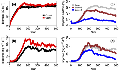
Figure 3. Applications of UVAFME-VOC to study ozone and climate warming impacts on forest dynamics and isoprene emissions over the 500 year s of forest dynamics initiated from bare ground. (a) elevated O3 impacts on the forest biomass (tC ha−1); (b) elevated O3 impacts on the isoprene flux (mg m−2 d−1); (c)–(d) show the impacts of two warming scenarios (+2 and +4 ˚C warming relative to the base climate) on the relative forest composition changes (%) for isoprene producers (c) and on the corresponding isoprene flux (mg m−2 d−1) (d). This model simulates isoprene emissions at an hourly time step on the basis of demographic processes at a yearly time step. These simulations are all conducted in the temperate deciduous forest at a site located at the southeastern United States. See the detailed modelling protocols in Wang et al (2016 2017), and Wang et al (2018). (a) and (b) Adapted from Wang et al 2016. CC BY 4.0.
Download figure:
Standard image High-resolution imageThis finding contradicts previous studies based on models that lack an explicit simulation of the species-specific sensitivity to O3 (e.g. Sitch et al 2007). With more isoprene production arising from increased presence of isoprene-emitting species, there is a positive feedback between tropospheric O3 and forest (figure 3(b)). Additionally, UVAFME-VOC was also applied to study climate warming impacts on forest isoprene emissions (Wang et al 2018). This latter study found that, unlike previous studies with aggregated models (Guenther et al 2006), climate warming will not always stimulate isoprene emissions. In addition to its direct enhancing effect, warming simultaneously reduces isoprene emissions by causing a decline in the abundance of isoprene-emitting species (figure 3(c)). This ecological effect eventually outweighs the physiological one, and reduces the overall emissions over time (figure 3(d)). These findings have significant implications for the understanding of complex climate-biosphere-air quality feedbacks. Results from an individual-based gap model are not congruent with those produced by more aggregated ecosystem models, and demonstrate the capability of gap models in addressing feedbacks between biosphere and atmospheric chemistry.
Estimating Amazon-wide biomass with local gap models—Linking remote sensing and forest modelling for large scale applications is a promising field in forest ecology (Shugart et al 2015). There are two options to link forest simulations with remote sensing: either by using remote sensing products to initialize existing forest models (e.g. using forest cover maps) or alternatively, using first forest models to explore relationships between different forest attributes (e.g. forest height and biomass) and apply them to remote sensing to derive hidden forest attributes that cannot be measured directly by remote sensing (like forest productivity or forest structure, Knapp et al 2018). The advantage of using an individual-based forest model is that it brings along information on forest structure (Fischer et al 2016). This structural realism can be used to link simulated and remotely sensed information on forest structure at different levels (e.g. canopy height). Rödig et al (2017) used remote sensing data to establish large-scale applications of forest gap models and to derive maps of forest carbon stocks and fluxes at the continental scale.
They used the forest gap model, FORMIND (Fischer et al 2016), which is normally applied at stand levels, to simulate forest dynamics at a much larger scale, here the Amazonian rainforest (figure 4). This large-scale application required two steps: (1) the technical implementation and (2) the regionalization approach. The technical application took advantage of modern high-performance computers and ran simulations with parallel computation. The regionalization approach involved the regional modification of model parameters for which a process-based description is often missing (e.g. mortality rates change in different regions, for example due to changes in environmental factors). With this parameter adaptation, simulation of heterogeneous forest dynamics can be achieved for the Amazon region. However, the estimation of these model parameters is a complex process and only a limited amount of forest site observations is available. Therefore, an inverse modeling technique for forest models was developed (Lehmann and Huth 2015).

Figure 4. High-resolution biomass map for the Amazon rainforest at 1000 m resolution (left) and relative frequency distributions at 40 m resolution (right) derived by linking FORMIND simulation results with remote sensing data. Rödig et al 2017. John Wiley & Sons. © 2017 John Wiley & Sons Ltd.
Download figure:
Standard image High-resolution imageThis technique has been used to calibrate model parameters against field inventory data, but it is potentially also applicable to automatically calibrate forest models with remote sensing data. To derive biomass maps and forest productivity maps across large landscapes with a fine resolution, they linked the forest gap model with Amazon-wide forest height maps from remote sensing, in the current case, the forest height map of Simard et al (2011). These canopy heights are used to identify successional stages of forests. The result was a map of forest biomass in the Amazon rainforest at 40 m resolution (Rödig et al 2017, figure 4). Beside forest biomass, gap models also provide information on the relations among successional stage, disturbance state and carbon fluxes (Fischer et al 2016). These findings highlight the capability of deriving high-resolution maps of carbon fluxes, as well as biomass, across large landscapes such as the Amazon forests system.
Additional carbon releases due to tropical-wide forest fragmentation—Another approach of large scale applications of forest gap models focuses on the influence of land use on tropical forests (figure 5). By combining remote sensing data and a forest gap model, Brinck et al 2017) calculated long-term carbon losses due to forest fragmentation. They analyzed the impact of edge effects on different forest-stand carbon fluxes using the FORMIND model (Pütz et al 2011). These results are combined with high-resolution forest cover maps. In detail, each forest fragment in the tropics was counted and analyzed using such tree cover maps (Landsat with 30 m resolution). Forest area lying within 100 m of a forest edge was evaluated, as wherein this forest edge area trees suffer increased mortality. The impact of this increased mortality on forest structure and dynamics was analyzed by field data (Laurance 2000, Laurance et al 2011) and by forest gap models (Pütz et al 2014). Combining high-resolution forest cover analysis with results of gap model simulations provides important findings, notably tropical forest fragmentation increases carbon loss significantly and should be accounted for in the global carbon cycle (Brinck et al 2017).
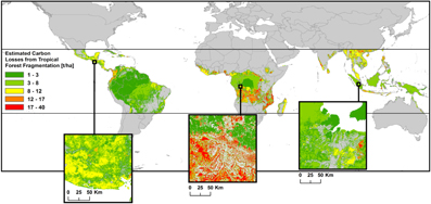
Figure 5. Worldwide carbon emissions due to fragmentation of tropical forests. Colors represent the estimated carbon losses for each forest fragment. Adapted from Brinck et al 2017. CC BY 4.0.
Download figure:
Standard image High-resolution imageUsing gap models to simulate global carbon fluxes from forests—The FORCCHN model (FORest ecosystem carbon-budget model for CHiNa model, Ma et al 2017) is a gap model designed for global applications involving forest structural change (tree height, leaf area index, size distributions of trees, successional dynamics, etc) and its influence on biogeochemical fluxes from forests. Its simulations are based on a plot-scale gap model, which plants, grows and kills the individual trees categorized into functional types rather than species.
The FORHCHN model assumes that net photosynthate is allocated to the tree growth, leaf litter and fine roots. Any remaining photosynthate is stored in a so-called 'buffer carbon pool' on a daily basis. At the end of the year, this cumulative 'buffer carbon pool' is primarily used to support the growth of canopy height and basal diameter increment of each tree on each simulated plot. As a preamble to applying the FORCCHN model to estimate global carbon uptake by forest ecosystems, Ma et al (2017) used the CO2 flux measurements from 37 eddy covariance flux sites located between ∼38°S to ∼70°N to examine the FORCCHN's performance. In these initial tests, model simulated higher correlations in gross primary production (GPP) for the 37 sites (correlations averaging 0.72 across predicted and observed daily across the 37 sites), ecosystem respiration (ER, average correlations of 0.70) and net ecosystem production (NEP, average correlations of 0.53) across all forest biomes.
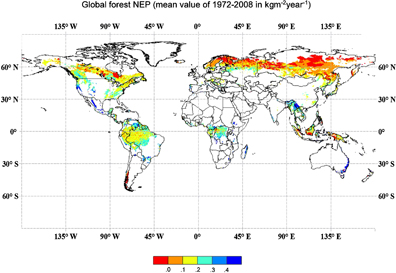
Figure 6. Global patterns of the average net ecosystem production (kg m−2 yr−1) for global forests from 1970–2008 as simulated by the FORCCHN model. Net ecosystem production is gross primary production minus ecosystem respiration. Note the red areas in the upper forest regions of the Northern Hemisphere, which indicate ecosystem carbon losses over this interval.
Download figure:
Standard image High-resolution image
Ma and his colleagues then applied the FORCCHN model to estimate the carbon fluxes on global scale with the satellite-derived data from IGBP-DIS land cover classification system and Global Land Surface Satellite LAI products. The simulated results are comparable to and reinforce estimates reported in other studies. More generally, these results also indicate that gap models, notably the FORCCHN model, have application in global carbon modeling. Figure 6 illustrates the performance of the FORCCHN model simulating the net ecosystem production for global forests over the interval 1970–2008. One significant pattern seen in this analysis is the region in the Eurasian boreal forest region where red colors indicate landscape- to regional-scale negative NEP across the very part of Eurasia that has been significantly warming over this time interval (Serreze et al 2000). One can also see similar negative NEP in tropical regions undergoing clearing that has yet to be offset by recovery.
When available, forest inventory data (i.e. tree height and basal diameter of individual tree on survey plots of an appropriate size.) are used as the initial conditions to start the FORCCHN model. As was just mentioned for Amazonian estimation of the components of biomass dynamics at the regional scale, in global applications a significant difficulty lies in the lack of availability of extensive plot-based inventory data. For this reason, satellite-derived LAI products (along with information on forest types, latitude, and elevation for a given plot area) are used to initialize the stand structure in the initial year of the simulation. For the FORMIND application for the Amazon (above) the procedures used are outlined in Rödig et al (2017) and Lehmann and Huth (2015). For the FORCHHN model, procedures in Zhao et al (2012) are used for initialization the states of the individual trees on plots. These applications could likely be improved by perfecting an observational basis for the initialization data. The availability of synoptic individual-tree inventory data for the world's forest at large scales is essentially non-existent and there are relatively few good national-scale examples. One can expect that with the deployment of LiDAR and RaDAR satellites by multiple international space agencies, the availability of better characterizations of forest physical structure will serve to improve initialization of spatially extensive gap-model applications.
Some of the parameters of some ecological process models embedded in the FORCCHN model have been applied globally. For example, to simulate vertical light distributions and soil conditions, FORCCHN is coupled with a forest-canopy-height radiation sub-model and a CENTURY (Parton et al 1988 and 1995) sub-model. These sub-models play a key role in photosynthesis and decomposition in the FORCCHN model. FORCCHN model uses such physiological and ecological functions along with the forest structure to describe the productivity of global forests. High-quality global-meteorological databases are imperative to construct the estimates of the local environmental factors for the global simulations.
Technological advances in remote sensing should improve the climate observations used in the FORCCHN model and other gap models. For the testing of these models more observation stations have established and can provide more extensive observational data, particularly for carbon flux data. The FORCCHN model can also consider the influence of CO2 concentration in the atmosphere on vegetation growth. The current FORCCHN simulation results can be compared directly with the station carbon flux data at the site scale directly, and is its basic validation for global modelling.
The global-scale modeling with IBMs and associated gap models does present have several challenges for data collection at different scales. Some of this regards a better characterization of species parameters and better functional representations of ecological process. These represent a continuation of ongoing silvicultural and biogeochemical research agendas. One hopes that the relative success in gap models when tested against a spectrum of forest properties can inspire a increased interest in these research areas.
Despite the advances in remote sensing technology, uncertainties remain and directly influence the vegetation initialization. For example, the FORCCHN model is initialized with two different sorts on information. First, the model requires individual-tree information—tree species, diameter, height, etc of each tree on a sample plot or alternatively a set of rules allowing the model to spin-up a theoretical forest landscape of a given age. Second, plot information is required—the tree numbers on the plot, leaf area index, available nutrients.
Since the impact of environmental change on forest ecosystem fluxes is not only limited to CO2 enrichment and climate change, but also to the cycling of different elements. Nitrogen (N) is a key element to photosynthesis process, which generates a corresponding problem of determining ecosystem-N fluxes and initializing N-storage. C and N are interactive and many studies have shown that atmospheric nitrogen deposition can affect the uptake of CO2 in the subtropical, temperate and boreal forests. The understanding of these interactive processes at multiple scales remains a challenge.
Relationship among gap models and other global modeling approaches
Global modeling approaches of the terrestrial surface of the Earth in response to concerns over 'greenhouse' gases and anthropogenic climate change have three originating pathways (see chapter 5 of Shugart and Woodward 2011):
- 1.Material transfer models—Approaches that are based on the transfers of carbon (and other elements) from compartments such as vegetation or soil to compartments such as the atmosphere or shallow oceans (e.g. The CENTURY model, Parton et al 1988–1993, the TEM model (Raich et al 1991). These models are inspired by pharmacological models that move chemicals from compartments such as muscle, bole, liver, etc in the 1930s (Teorell 1937, Sheppard and Householder 1951). They have been under continual development since.
- 2.Canopy process models—Models that begin with the biophysics of plant canopies with respect to fluxes of heat, along with CO2, H2O and other compounds to determine the response of plant process to environmental changes. They represent the canopy as a single or multi-layer unit with a fixed structure (i.e. leaf area). Photosynthesis and transpiration are simulated by estimating microclimatic variation and stomatal conductance for the canopy (or canopy layers). Some models in this broad categories are focused on heat and water transfers and are used to couple the atmosphere to the land surface in general circulation models (e.g. Bonan et al 2002); others have found application in the heat, water vapor and CO2 fluxes measured at eddy-correlation-based micrometeorological studies (e.g. Baldocchi 2003). Many of these models have an embedded biochemical model (e.g. Farquhar et al 1980) to couple biological features of the canopy to the atmosphere under given environmental conditions.
- 3.Biogeographical models—Since the early writings of Theophrastus, the 4th Century BCE Greek philosopher, ecologists have been concerned with the interactions between climate and plant distributions. Alexander von Humboldt formalized the interaction among vegetation, climate and the environment. He was followed by a progression of Germanic biogeographers—Grisebach with the first global vegetation map in 1872; Schimper with the first vegetation map with modern biomes in 1898; Köppen with a global climate map tied to vegetation in 1930 (see: chapter 1, Shugart and Woodward 2011). In applying biogeographical models, one seeks to use the current vegetation/climate relationships as a basis for remapping the potential vegetation (Küchler and Zonneveld 1988) expected under a changed climate. The mapping of global vegetation faces a philosophical challenge on the level of abstraction used. Vegetation can be mapped globally by vegetation/climate relations (e.g. Emanuel et al 1985); by life form or functional type by collecting species into categories (tropical evergreen trees, deciduous temperate trees, etc), mapping the vegetation/functional types each on to climate conditions and then assembling the expected vegetation from all the functional types that could occur under a given climate (Box 1981); by species niches that map species' presence and absence onto climate variables and then assemble the expected combination of species sharing the climate at a particular location to produce an expected vegetation (e.g. Iverson et al 2008).
Currently these approaches (or a subset thereof) are melded to produce dynamic global vegetation models (DGVMs), which are used to assess the global vegetation consequences of climatic and other global changes.
Dynamic global vegetation models
DGVMs, for example, a globalized version of the TEM (McGuire et al 1992) model, BIOME-BGC (Running and Hunt 1993), a global version of CENTURY (Parton et al 1993), CASA (Potter et al 1993), IBIS (Foley 1994), SiB2 (Sellers et al 1996), LPJ (Sitch et al 2003), ORCHIDEE (Krinner et al 2005), et al have been regularly exercised in comparative model experiments for current conditions and changed global environmental conditions. Across many of these model comparisons, the models produce results that are similar one-to-another with respect to global heat, water and carbon fluxes. They depart from one another under altered climate conditions and particularly do so under alterations in the global concentration of atmospheric CO2 (Shugart and Woodward 2011). Much of this arises from differences in formulation/conceptualization of some fundamental processes in the models and from our lack of information on how some of these processes vary spatially across scales.
DGVMs are usually deployed on global grids on the order of 0.25° × 0.25° latitude-longitude cells. The averaging of physiological process across such cells to a bulk homogenous representation is confounded by scaling challenges, notably with respect to canopy processes, the allocation of material to different plant tissues, the inclusion of heterogeneous drivers such as wildfire, etc. The networks of eddy correlation observation sites provide important adjunct data for the testing and parameterization of these models. This is the reason why the FORCCHN model, which was discussed above, was compared to such site data in the Ma et al (2017) paper.
Ecological models evolve as more is learned and as their performances are evaluated. The recent gap models that we have presented as examples in the sections above perform well in tests against flux sites, which implies their suitability to represent biological and ecological processes at larger spatial scales. Allocation of carbon to tissues in a forest as a whole is a consequence of the summation of carbon allocation by myriads of single plants each controlled to some degree by its situational context. One of the aspects that gap models bring to understanding the global carbon budget is a direct representation of vertical and spatial heterogeneity.
Fused function and structure models
An underlying assumption in some DGVMs has been the issue of how scaled-up ecosystem processes such as gross and net primary productivity, or ecosystem respiration can include the effects of the physiognomic differences in ecosystems in different stages of recovery from disturbances or across heterogeneous landscapes. This difficulty is intrinsic in some of these formulations. In the simplest sense and as an example, gross primary productivity (GPP) increases with light regularly if it exceeds a certain amount of light (the compensation point). As light increases, it becomes asymptotic to the maximum assimilation rate (Amax) of CO2 into the photosynthesis process. Because this asymptotic change is non-linear, the average GPP summed for an assemblage of leaves (or trees or stands or landscapes) under a range of conditions is not necessarily the response of an average leaf under the average of that range of conditions.
Generally, the formulations of some of the processes in DGVMs are conducted under an assumption that the functions describing the processes at a small scale are of the same functional form when summed to a larger scale—with only the parameters needing to be adjusted. This seems a strong assumption given for the lack of the additivity property for nonlinear systems. Forest ecology, starting with A.S. Watt (1947), strongly endorses the concept that biomass dynamics at a scale of ∼0.1 ha operate in a quasi-periodic cycle with biomass increasing with tree growth, then dropping abruptly with the death of the dominant tree and the repeating the growth phase. The summation of these to a landscape dynamic composed of such elements and reaches a quasi-equilibrium perhaps with an overshoot of the eventual quasi-equilibrium (Bormann and Likens 1979). These different behaviors, which are frequently seen in gap models (Shugart et al 2010), implies that the functions underlying forest biomass dynamics does not scale with the additivity property.
Much of these difficulties arise from the effects of changes in the forest structure (numbers of trees of different species and sizes), particularly with the advent of airborne and satellite systems capable of measuring the structure of forests using different combinations of high resolution imagery and RaDAR and LiDAR systems (Shugart et al 2010). A straight-forward approach to this problem is to allow a gap model (or other individual-based model) to drive the changes in the structure of the forest under the constraint that the net productivity from the individual-based models 'agree' with an aggregated process models running in parallel.
Friend et al (1993) took this approach to meld the capability of the ZELIG gap model (Urban et al 1991) to produce spatial forest structure with that of the FOREST-BGC (Running and Coughlan 1988) model to produce transpiration and water budget and the PGEN model (Friend 1991) to simulate detailed photosynthesis and water-use of individual trees. The resultant model, HYBRID, was then applied to simulate daily canopy photosynthesis and soil water under for different forest in Missoula, Montana and Oak Ridge, Tennessee. A significant analysis of the sensitivity of the simulated NPP to factors such as CO2 concentration, precipitation, temperature, etc was conducted for sites in both locations. One significant finding from the point of view of scientist working with gap models was the HYBRID model's demonstration that one could incorporate altered CO2-levels with a physiologically detailed model into a gap model, which was a topic of spirited discussion at the time. Now at version number HYBRID4 (Friend and White 2000), this approach has become a significant contributor to ongoing assessments of the global carbon cycle (Thurner et al 2017).
Ecosystem demography models
One can also describe the state of a forest based on size class categories of trees. The number of individual trees in a size class change with death removing trees from a size class, growth moving trees from one size class to the next and birth inserting new trees into the smallest size class. Since tree size classes can be used to estimate the average biomass or carbon content of the average tree in each size class, these models can also predict net primary production. Korzukhin and Antonovski (1992) used a similar approach, implemented as integro-differential equations, to solve for structure and productivity in Russian boreal forests. Kohyama (1992, 1993) used a partial differential equation model to simulate changes in forest structure for a tropical rain forest in Borneo (discussed above).
Another important such application to tropical rainforests is that of Moorcroft et al (2001), who parameterized a gap model for an Amazonian rainforest using a postulated relationship between growth rate, photosynthesis and wood density. The resultant model was used to parameterize a statistical model of the size distribution of trees across the Amazon Basin using the approach pioneered by Kohyama (1993) to represent forest structural dynamics as a partial differential equation in time, numbers of trees, and tree size. The partial differential equation model provides canopy structure to constrain the results produced by a photosynthesis model. This model, called the Ecosystem Demography (ED) model, has found application to summarize the demography of mosaic forests over large areas (Amazonia). The ED Model represented the Amazonian forests as a Kohyama-type partial differential equation of numbers versus size of trees and use a gap model to estimate the growth (the forward vector with respect to the size axis) and mortality (the downward vector). These are constrained by photosynthesis rates using a DGVM photosynthesis/respiration model. This approach of letting a net productivity model constrain tree growth and demography was at the core of the earlier HYBRID model (Friend et al 1993) that was discussed above.
Performance and prospects of gap models in global change assessment
In concluding, it is logical to discuss the current and future use of gap models and other IBMs in global studies. At present, gap models appear capable to reproducing forests and forests change with fidelity equivalent to DGVMs in duplicating the components of carbon fluxes measured at the worldwide networks of flux towers. As this review indicates, they have found application at a local landscape-level, through regional and to global predictions with respect to environmental change assessment and to atmospheric and terrestrial surface feedbacks at these scales. They have the advantage of producing expected forest structures, which provide the opportunity to test the model prediction against the future observations that will come from a new generation of Lidar, RaDAR and other technologies of satellites (Shugart et al 2015).
Their predictions of forest composition can be tested under evaluations of forest composition from paleoecology, which provides gap models access to hypothetico-deductive testing—often a challenge in testing DGVMs. Evaluation of the biogeochemical consequences of disturbances in generally straight-forward, at least conceptually in gap models and other IBMs. However, DGVMs have an intrinsic advantage in simulating multiple biomes—forests, grasslands, deserts, etc. One can 'tune' the physiological performance of the bulk representations of physiological processes involving elemental fluxes, much more effectively in DGVMs, but a question remains as to whether a tuned model can be expected to perform outside its domain of calibration.
What are the future challenges? There are several significant issues in the continuing development of gap models. While there are several spatially explicit gap models and there were also spatial models among the earliest IBMs, spatial processes remain a challenge. There is a range of spatial interaction in spatial IBMs ranging from gridded mosaics of a gap model simulating each grid-element to truly spatial models with two- and three-dimensional interactions among individual trees. An attendant problem involves the need to replicate simulations of the multiple realizations of spatial IBMs and determining how these patterns can be tested against reality. Large-scale spatial phenomena such as plant migration are both difficult to parameterize and to implement in models.
Model experiments investigating the effects of different numbers of species and/or functional types in a model would be valuable. The development of IBMs for the transition zones between, for example, forest and grasslands or forest and savannahs is a difficult and significant problem. A better characterization of the ecological and performance of tree species would be invaluable at this time.
For all of this, gap models and related IBMs have made a significant contribution to our understanding of potential ecosystem dynamics at different spatial scales and over all the forested continents. There is clearly work to be done, but the use of these models to illuminate global environmental issues provides promise—particularly in an era of increased computation and observational capability. That the consequences of global change and its change of the surface for humankind is at hand is certainly ample motivation.