

Abstract
Accurate, consistent reporting of changing forest area, stratified by forest type, is required for all countries under their commitments to the Paris Agreement (UNFCCC 2015 Adoption of the Paris Agreement (Paris: UNFCCC)). Such change reporting may directly impact on payments through comparisons to national Reference (Emissions) Levels under the Reducing Emissions from Deforestation and forest Degradation (REDD+) framework. The emergence of global, satellite-based forest monitoring systems, including Global Forest Watch (GFW) and FORMA, have great potential in aiding this endeavour. However, the accuracy of these systems has been questioned and their uncertainties are poorly constrained, both in terms of the spatial extent of forest loss and timing of change. Here, using annual time series of 5 m optical imagery at two sites in the Brazilian Amazon, we demonstrate that GFW more accurately detects forest loss than the coarser-resolution FORMA or Brazil's national-level PRODES product, though all underestimate the rate of loss. We conclude GFW provides robust indicators of forest loss, at least for larger-scale forest change, but under-predicts losses driven by small-scale disturbances (< 2 ha), even though these are much larger than its minimum mapping unit (0.09 ha).
Export citation and abstract BibTeX RIS

Original content from this work may be used under the terms of the Creative Commons Attribution 3.0 licence.
Any further distribution of this work must maintain attribution to the author(s) and the title of the work, journal citation and DOI.
Corrections were made to this article on 15 January 2018. The citation year was amended.
1. Introduction
Since 2000, forest loss globally is >2.53 million km2, with net losses concentrated in tropical regions (Hansen et al 2013). The release of CO2 to the atmosphere driven by tropical land-cover change has been estimated to be 2.0 ± 1.1 PgC yr−1 (Grace et al 2014), predominately driven by this deforestation (Le Quéré et al 2014). Monitoring forest change is therefore critically important; under the Paris Agreement (UNFCCC 2015) and through REDD+, countries are required to document and record changes in forest extent on a frequent basis, ideally at least biennially (GFOI 2016), in order to assess levels of deforestation-driven greenhouse gas emissions (Gibbs et al 2007, Stickler et al 2009). The recent development of open, globally consistent and regularly updated forest loss datasets, following the incremental release of open satellite data through this century, has huge potential in facilitating this monitoring, particularly for countries that lack the capacity to develop independent forest monitoring and reporting systems (Goetz et al 2015). For example, the Landsat 7/8 archive has been exploited to produce an annual 30 m resolution map of global forest change from 2000–2014 (referred to here as Global Forest Watch, GFW) (Hansen et al 2013); similarly, but at a coarser 500 m resolution the MODIS-based Forest Monitoring for Action (FORMA) product provides sub-monthly estimates of deforestation (Wheeler et al 2014). These data could be used directly by countries to save them creating their own system (GOFC-GOLD 2014, GFOI 2016); they also have an obvious utility in validation by the international community, and for assimilation into earth system models (Bloom et al 2016).

Figure 1. Map indicating the location of the Acre site (a) and Rondonia site (b).
Download figure:
Standard image High-resolution imageAn important challenge in the successful inclusion of these data within national Measurement, Reporting and Verification (MRV) frameworks is to understand both the accuracy with which this change is reported, and the degree of associated bias. While we believe the methods used and overall statistics produced are useful and valid, at regional and national levels, global algorithms could under- or over-report changes, if differences in, for example, forest structure, or the pattern of deforestation, contribute towards a variations in their performance (e.g. Tropek et al 2014, Achard et al 2014). This may lead to systematic biases in reported rates of change, when aggregated across a region. However, it is also possible that such products allocate change to the wrong year, or detect erroneous patterns of change, when compared to reality. We thus do not know the extent to which algorithms produced at a global scale can produce unbiased change estimates at a national scale.
Here, we test the bias and accuracy of these global products in two contrasting sites within the Brazilian Amazon, and compare them to Brazil's national forest change product, PRODES (INPE 2015). These sites are chosen for two reasons. Firstly they are both areas experiencing rapid rates of forest loss, but the rates, styles and underlying drivers of deforestation vary; these sites therefore provide an opportunity to test the extent to which these factors influence the performance of satellite-based detection of forest loss. Secondly, we focused on sites in Brazil because it has the longest running and most trusted national forest monitoring system: other countries would need a significant investment to produce similar systems. It therefore represents a good test case as to whether global datasets provide comparable information. Like GFW, PRODES is based on analysis of the Landsat archive; however, whereas the changing forest extent indicated by GFW is mapped using an automated process, PRODES is produced using semi-automated software tuned to Brazil, with heavy manual involvement by a large team of interpreters. The ability of these products to detect forest loss is assessed against an independent time series of annual forest loss derived from annual 5 m resolution RapidEye imagery using supervised classification and spanning 2009–2015 at both sites.
2. Methods
2.1. Study sites
The first validation site spans ∼2100 km2 in northern Acre province (figure 1). Deforestation, primarily driven by selective logging in concessions followed by small-scale agriculture, has gradually expanded into undisturbed forest following a classic fishbone pattern that radiates out from the road network (Southworth et al 2011) (figures S1, S2). The second site is located in Rondonia (figure 1) and covers ∼2500 km2. Deforestation in this locality is characterised by large scale clearances and widespread clearing and conversion (using fire) to agriculture (largely soy bean) and pasture (Rodrigues-Filho et al 2015) (figures S3, S4).
2.2. Data
2.2.1. RapidEye data processing and classification
For both sites, high-resolution (5 m) five-band RapidEye scenes were obtained for every year within the timespan 2009–2015 (table S1). The sites were chosen based on the availability of cloud-free RapidEye scenes, however inevitably there were still some cloud cover problems. Where possible we used scenes that spanned the entire reference sites, but if this was not possible, multiple scenes were stitched together so that the coverage for the year was as close to 100% as possible.
Each RapidEye scene (or partial scene) was independently classified into regions of forest and non-forest using a Support Vector Machine algorithm in ENVI 5.1. Specifically we used two pyramid levels, a radial basis function and three classes—forest, non-forest (vegetated), non-forest (un-vegetated). The SVM classification utilised all five available bands (RGB, Red-edge, NIR), with the classes characterised by a manually defined training dataset comprising at least 20 Regions Of Interest (ROIs) and 20 000 pixels. For images containing smoke, haze or cloud, affected areas were masked using a manually selected Haze Optimisation Threshold (Zhang et al 2002). Areas identified as cloud, haze or smoke were subsequently buffered by a user-defined radius. Cloud shadow was straightforward to isolate as an additional class in the SVM. The two non-forest classes were merged into a single non-forest class.
Following initial classification, the thematic land-cover maps were spatially filtered using a 7 × 7 pixel (1225 m2) moving window, with the final classification determined by the most likely classification based on the combined posterior probabilities. The thematic maps were then compiled into land-cover change trajectories spanning 2009–2015. For pixels where overlap between partial scenes occurs within a given year, we classify any cloud-free pixels in order to constrain the date of forest change as much as possible; however this only represents a small subset of the dataset. To reduce further misclassifications arising from the spectral similarity of some forest and vegetated non-forest pixels, these land-cover trajectories were temporally filtered so that for a change to be accepted, it had to be corroborated across two successive images. This filtering process limits the extent to which small disturbances (i.e. degradation) can be detected; however, without extensive field constraints it is difficult to distinguish degraded forest based solely on optical imagery (Asner et al 2005, Lambin 1999, Olander et al 2008); these disturbances would be missed in any case in coarser products.
As there is a mismatch between the RapidEye acquisition dates and the annually incrementing timestep of GFW and PRODES, in the best case (cloud-free coverage) the temporal window within which it is possible to constrain the timing of forest loss encompasses the period between successive RapidEye scenes; it is not possible to isolate forest loss to a single year. This effect is compounded for pixels where there is cloud cover obscuring a pixel across the time period where forest loss occurred. The RapidEye-based land-cover trajectories are therefore presented as a range of possible dates of deforestation bounded by the dates of the scenes between which the change occurred (figure 2); this encapsulates the uncertainty associated with the timing of forest loss. GFW and PRODES are assumed to indicate the correct timing of forest loss if this is recorded within the temporal constraints provided for that pixel.
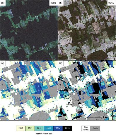
Figure 2. RapidEye images depicting shifting forest extent between 2009 (a) and 2015 (b) for a portion of the Rondonia site. Associated maps of forest loss indicating earliest (c) and latest (d) possible year of forest loss based on the classified RapidEye scenes. Maps for the full Rondonia site and Acre site are available in the supplementary information (stacks.iop.org/ERL/12/094003/mmedia).
Download figure:
Standard image High-resolution imageThe spatial accuracy of the reference data was assessed using a manual point check following a stratified random sampling approach (Olofsson et al 2014) for a three-class thematic map (stable forest, non-forest, and forest loss) covering the full time period. This provided bias corrected estimates of class areas and their associated standard errors, alongside estimates of overall accuracy, and rates of omission and commission errors (Olofsson et al 2014). For forest loss between 2010 and 2014 (the crossover period with GFW) the overall accuracy of the RapidEye reference product was 98.7 ± 0.5% for Acre and 94.2 ± 1.0% for Rondonia. The respective commission error rates for mapped forest loss at these sites were 13.3 ± 4.0% and 9.8 ± 3.1%; likewise the respective omission error rates for mapped forest loss over the same period were 17.0 ± 10.0% and 16.1 ± 3.4%. Full accuracy statistics and confusion matrices for the reference data are tabulated in the supplementary material (tables S2–S4).
2.2.2. GFW, PRODES and FORMA forest loss data
30 m resolution maps of progressive forest loss were produced from the GFW data for the years 2010–2014 (Hansen et al 2013). The initial segmentation of forest/non-forest area was generated using the GFW tree cover map for the year 2000, using a tree cover threshold of 30% (UNFCCC 2001, Morton et al 2011), from which we removed subsequent forest loss prior to 2010. Areas flagged as regrowth were ignored, as there is no corresponding temporal information, and the timing of afforestation is inherently challenging to pinpoint (Hansen et al 2013). PRODES provides comparable maps of progressive forest loss (INPE 2015). We noted a small (∼250 m) systematic offset between PRODES and the other data. While insignificant at a regional level, this offset would have significantly impacted on the subsequent pixel-wise comparison, so we corrected this offset using a linear translation. For forest loss estimates for FORMA (Wheeler et al 2014), the bi-monthly alerts (pixels highly likely to have experienced large-scale clearance) were resampled into a monthly resolution product, in which the area of forest loss mapped was estimated according to the number of alerts multiplied by the pixel area; initial forest extents were assumed to match those indicated by GFW.
All datasets were re-projected and resampled using a nearest neighbour approach, so that they matched the corresponding projection (UTM) and resolution (5 m) of the RapidEye reference data. Full maps of progressive forest loss for each dataset are included in the supplementary information (figures S1, S2—Acre—and S3, S4—Rondonia).
2.3. Spatiotemporal accuracy assessment
The spatiotemporal accuracy of GFW and PRODES was assessed based on a two-step procedure: (i) spatial accuracy is assessed with a pixel-pixel comparison, leading to the marking of correctly identified change, no change and errors of omission and commission (Olofsson et al 2014) (figure 3); (ii) for pixels correctly identified as changing within the time series, temporal accuracy was determined by comparing the date of change indicated by each product with the range of possible dates constrained by the RapidEye reference data. If the change occurred within the constraints provided, it was given a lag of zero. Note that resolution differences between the published products (30 m resolution GFW, 60 m PRODES and 5 m RapidEye) will generate errors around the margins of correctly identified disturbances, inevitably degrading the reported spatial and temporal accuracy of the GFW and PRODES products. Due to the larger resolution differences, we do not extend the pixel-wise analysis to include FORMA. To assess the relative performance with respect clearance size, we discretised the annual change maps into distinct disturbances and calculated the accumulated area of forest loss contributed according to the size of the disturbance.
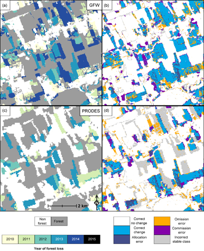
Figure 3. Maps of forest loss for the same portion of the Rondonia site depicted in figure 2 based on GFW (a) and PRODES (c), alongside a pixel-wise comparison of forest loss for both GFW and PRODES relative to the RapidEye reference data. The proximity of omission, commission and allocation errors close to correctly identified forest loss are at least partly a result of the resolution difference between GFW, PRODES and the reference RapidEye scenes. Note that GFW includes forest loss up to the end of 2014, while PRODES includes forest loss up to the end of 2013. Full maps for both sites are presented in the supplementary information.
Download figure:
Standard image High-resolution image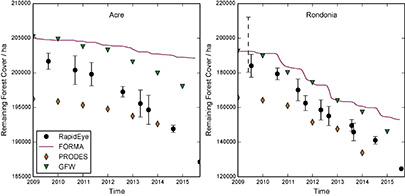
Figure 4. Comparison of forest cover trajectories indicated by four different deforestation products: RapidEye time series, FORMA, Global Forest Watch Forest Loss (GFW) and PRODES. Vertical offsets are a consequence of varying estimates of initial forest area associated with each product. Error bars in the RapidEye time series indicate the range of forest cover indicated at each time step according to the temporal uncertainty in the land-cover trajectories for each pixel (i.e. accounting for the earliest and latest possible date of change).
Download figure:
Standard image High-resolution image3. Results
At the site-level, the mapped land-cover trajectories vary significantly between forest loss products (figure 4). Discrepancies arise due two factors. Firstly, there are marked differences in initial forest extent, generating systematic offsets in the initial conditions. GFW estimates much greater initial forest cover than the RapidEye analysis, whereas PRODES has a smaller estimate. Secondly, while all products reveal a reduction in forested area at both sites, rates of loss indicated vary considerably. For the period covered by the RapidEye time series, bias corrected estimates of forest loss (calculated following Olofsson et al 2014) indicate deforestation rates of 2060 ± 160 ha yr−1 for the Acre site and 9440 ± 360 ha yr−1 for the Rondonia site. In contrast, the rates of forest loss indicated by the other forest loss products are lower (table 1) indicating a systematic bias that acts to under-estimate the extent of forest loss in both regions. At both sites, the rate of forest loss increased between the 2014 and 2015 images (figure 4); GFW terminates in 2014, while PRODES terminates in 2013. Using linear interpolation to truncate the RapidEye time series at the terminating dates of the other products, the apparent bias at the Acre site is −27 ± 8% (−230 ha yr−1) when using GFW, and −49 ± 8% (−760 ha yr−1) when using PRODES. Conversely, at the Rondonia site, the respective biases are smaller, −4 ± 4% (−332 ha yr−1) for GFW, and −15 ± 4% (−1360 ha yr−1) for PRODES. In both settings, the rates of change indicated by GFW are closest to the RapidEye observations.
Table 1. Comparison of forest loss indicated by RapidEye time series, GFW and PRODES. Bias corrected means and 95% confidence intervals for the RapidEye forest loss extents are calculated based the good practice framework outlined by Olofsson et al (2014). A full summary of the accuracy statistics from a pixel-wise spatial accuracy assessment (table S2) is provided in the supplementary information. Percentage forest loss is expressed in terms of the total site area.
| Site | Acre | Rondonia | |
|---|---|---|---|
| Site Area/ha | 210 900a | 254 000 | |
| Rate of Forest Loss/ha yr−1 | RapidEye | 2060 ± 160 (0.98% yr−1) | 9440 ± 360 (3.729% yr−1) |
| GFW | 1320 (0.63% yr−1) | 8730 (3.43% yr−1) | |
| PRODES | 800 (0.38% yr−1) | 7570 (2.98% yr−1) | |
| FORMA | 490 (0.22% yr1) | 6600 (2.60% yr−1) | |
| Overall Accuracy compared to RapidEye | GFW | 95.2% | 87.2% |
| PRODES | 94.2% | 84.0% | |
aFor Acre site, the stated area excludes a 250 m buffer around the trunk channel that was not used in the assessment (see methods).
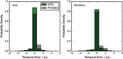
Figure 5. Temporal comparison for correctly identified forest loss in the period 2010–2014. Negative temporal errors indicates pixels in which forest loss detected by GFW and PRODES precedes the RapidEye classification time series; positive values indicate a lag relative to the RapidEye data.
Download figure:
Standard image High-resolution imageThe whole-period, area-averaged figures discussed above do not account for spatiotemporal errors, for example late reporting of change, or where incorrect detection of forest loss in one area is balanced out by an omission to report a forest loss elsewhere. Though data are normally used as area-averaged statistics, spatiotemporal errors can cause significant biases in the longer term, and when spatial (e.g. stratifying deforestation by forest type) or temporal (e.g. estimating trends in Activity Data for R(E)L calculations) subsets are used. The results of the spatial accuracy assessment indicate relatively good agreement between the forest loss indicated by GFW and the RapidEye time series (table 1, for a full summary of the pixel-wise accuracy statistics, see table S5). This agreement is further attested to by a visual comparison of the mapped forest loss, which shows a close correspondence between the patterns of disturbance indicated by each product (figure 3, also figures S1-S6). At the Acre site, disagreement for both stable classes and forest loss was particularly prevalent around the town of Manoel Urbano, in the NE quadrant (figure S2). Overall accuracy (i.e. compared to RapidEye 'truth' data) of the 2010–2014 GFW map of forest loss exceeded 95% for the Acre site, and 87% for the Rondonia site. GFW tended to outperform PRODES, particularly at the Acre site (tables 1, S5). We note here that the accuracies reported are derived from a comparison against the wall-wall maps produced from the RapidEye data, which in turn carry their own uncertainties (table S2). Given that a high spatial correlation of errors across datasets is unlikely, the aforementioned accuracies are likely to be lower bound estimates of their true accuracy.
Comparing pixels for which both GFW/PRODES and the reference data are in agreement that there is change within the period 2010–2014, both GFW and PRODES do well at correctly locating the change in time within the constraints provided by the RapidEye-based data (figure 5). GFW is particularly good in this regard, with 87.6% and 83.8% of the pixels for which change is correctly identified in space also, as far as we can tell, correctly located in time for the Acre and Rondonia sites respectively. PRODES does not perform as well, with only 75.6% of the matched forest loss allocated to the correct year at the Acre site, and 79.3% correctly allocated at the Rondonia site. Temporal errors are skewed to positive lags (a tendency to report change late), particularly at the Rondonia site (figure 5).
4. Discussion
We tested the accuracy of three forest loss products: GFW, PRODES and FORMA in two contrasting parts of the Brazilian Amazon by comparing against a higher resolution product derived from a time series of RapidEye scenes. While the general spatial patterns of change indicated by these products were consistent with the RapidEye reference data, there were notable discrepancies concerning: (i) the forest extent at the start of the period of interest—2009; (ii) rates of forest loss through 2009–2014 (figure 1). Comparing across sites, the performance of both GFW and PRODES is notably better for the Rondonia site relative to the Acre site; in particular, the Acre results are characterised by higher rates of omission errors for mapped forest loss.
Discretising the annual change maps to produce clearance size distributions, the impact of clearance size becomes immediately apparent (figures 6 and 7). Rates of forest loss at the Rondonia site are almost four times greater than the Acre site, with the style of deforestation dominated by the clearance of large fields (figures 3, 4 and S3, S4). Correspondingly, a much larger proportion of the cumulative forest loss mapped from the RapidEye time series is contributed by large forest disturbances with areas >10 ha (figure 6). Both GFW and PRODES indicate relatively close agreement with this in terms of the cumulative area contributed by these larger clearances at this site. Conversely, the Acre site is characterised by disturbances that are frequently smaller—the vast majority <10 ha in area (figure 7), with the gradual fleshing out of fishbone deforestation patterns characteristic of logging concessions (figures S1, S2, S5 and S6). At these smaller size classes, particularly <2 ha, GFW and PRODES do not detect the same level of disturbance to the forest (figure 7). Since these contribute overwhelmingly to the overall disturbance budget, the rates of change suggested by GFW and PRODES are particularly discordant with those suggested by the higher resolution data at the Acre site (figure 4). This effect is magnified when moving to FORMA, the coarsest product assessed.

Figure 6. Cumulative area of disturbance at the Rondonia site contributed by canopy clearances of different sizes for (a) and (b) RapidEye reference data, (c) GFW and (d) PRODES. The colour scheme indicates the year in which the detected forest loss occurred. The small peak in cumulative area in the highest PRODES size class arises due to an amalgamation of several large fields.
Download figure:
Standard image High-resolution image
Figure 7. Cumulative area of disturbance at the Acre site contributed by canopy clearances of different sizes for (a) and (b) RapidEye reference data, (c) GFW and (d) PRODES. The colour scheme indicates the year in which the detected forest loss occurred.
Download figure:
Standard image High-resolution image
The above comparison is significant in that it demonstrates that the performance of large scale deforestation products like GFW (and PRODES) varies dependent on the style of disturbance: the suggested negative bias is likely to be particularly marked in regions where deforestation is dominated by small-scale clearances. In making these comparisons, it is necessary to consider the Minimum Mapping Unit (MMU) of the products under assessment. In the case of PRODES, the MMU is 6.25 ha; the effect of this on the retrieved clearance area distributions is clearly evident in the abrupt drop-off in the area of cumulative forest loss below this threshold (figures 6 and 7). The larger MMU in PRODES accounts for a significant component of the omission errors, and the performance is improved for larger size classes (figures S2 & S6). In contrast, the MMU for GFW is 0.09 ha; negative biases for clearance classes <2 ha are therefore likely to be driven by limitations in the detection algorithm, rather than occurring predominately as a consequence of the MMU.
In general, temporal agreement between the forest loss products is good where there is agreement that forest loss occurred within the period of interest (figure 5). Lags may arise due to cleared fields being missed in the year during which forest was felled, for example if subsequent Landsat scenes were obscured by cloud cover or smoke. However, lags would also be expected given that the resolution of RapidEye imagery permits the detection of smaller scale and magnitude disturbances (figures 6, 7). It is only as these clearings are subsequently expanded in size or intensity that such changes can be detected with coarser resolution products. Late detection of forest loss early in the study period may also be responsible for some of the commission errors observed, and is consistent with the particularly high commission error rate in 2010 observed for GFW at both sites (figure S7). Some allocation errors will also be an inevitable artefact of differing resolution, since logged areas tend to propagate out from existing clearances. This likely accounts for most of the rare negative lags (reporting a change early), where change is mapped in PRODES or GFW before it is observed in the RapidEye scenes (although GFW may use changes in the annual vegetation cycle to detect subtle changes).
Given the pressing requirement for countries to report on changing forest extent on a regular basis (Stickler et al 2009, Gibbs et al 2007), wall-to-wall forest loss products such as GFW and PRODES are likely to be integral in such efforts. We would not recommend that FORMA is used in such accounting procedures due to its biases; however, this product is still very useful in providing near real-time alerts regarding deforestation activity. The results presented here indicate that the patterns of change detected by GFW and PRODES are consistent with changes observed with 5 m resolution imagery, but with a negative bias that is particularly prevalent at small clearance sizes. At the Acre site, the apparent bias suggests a significant amount of forest loss is being missed by both products (−27 ± 8% for GFW; −49 ± 8% for PRODES), whereas at the Rondonia site, the respective biases are smaller (−4 ± 4% for GFW; −15 ± 4% for PRODES), GFW in particular providing a close agreement in terms of overall rates of forest loss. Accounting for these biases will therefore form an important component of future attempts to integrate these products into inventories of regional forest change. Moreover, our results suggest that in areas of deforestation driven by a mosaic of small clearances (like our Acre site), a correction factor of +∼25% should be added to GFW and +∼50% to PRODES, to produce comparable change estimates to those produced with 5 m data. Where large clearance dominates, correction factors of +∼%5 and +∼15% respectively are suggested (based on Rondonia). Clearly these are only preliminary, and given the variability observed across these sites, extrapolating these bias estimates carries great uncertainty. Therefore we strongly suggest that further work is required to better constrain these estimates based on the parameters of disturbance.
Finally, it is important to note that while they have been reported as such, the differences between products are not necessarily 'errors', but may relate to differing definitions and aims. GFW, FORMA and our RapidEye reference data have a similar basic philosophy of mapping forest in each period and assuming pixels that have changed class from forest to non-forest permanently have been deforested. PRODES, however, is designed to map the first deforestation event of patches of intact forest, and therefore should not detect deforestation in areas that have previously been deforested, even if that disturbance occurred in the 1970's. This issue of definition of forest and deforestation is vital when comparing products, and using them to calculate Activity Data (GFOI 2016). It will become more vital still when the next generation of products for MRV and R(E)L incorporating degradation appear, as the definition of degradation is far less well defined than that for deforestation.
5. Conclusions
To conclude, of the three remote sensing products, GFW provides the closest match to the forest loss indicated by the RapidEye reference data. In part this highlights the benefits of the increased resolution of the Landsat-based products compared to MODIS-based FORMA (Hansen et al 2008); however, rates of deforestation mapped by PRODES are systematically lower than GFW at both sites, despite being based on the same satellite source data and with mapping methods tuned to the Brazilian Amazon (though these may partly relate to differing definitions of forest and deforestation). These differences are particularly marked in the Acre site, where the scale of disturbance is typically much smaller; in contrast, in the Rondonia site, the rates of change indicated by all products are more comparable. This indicates that the accuracy of these products is affected by the mode and scale of disturbance: large clearances are easier to detect at all resolutions. In many forests, biomass loss is driven by more subtle processes of degradation that are not straightforward to detect using optical sensors, even at 5 m resolution (Collins and Mitchard 2015). In order to include the impact of degradation in forest inventories, it may be advantageous to fuse optical products like GFW with complementary remote sensing approaches, such as radar (Mitchard et al 2011, Collins and Mitchard 2015, Reiche et al 2016, Le Toan et al 2011), that are more sensitive to disturbance that does not involve full canopy clearance.
Moreover, the results shown here indicate a positive outlook for the incorporation of GFW data into regional and national forest inventories (Goetz et al 2015), attempts to model changing carbon stocks at regional and global scales (Bloom et al 2016, Le Quéré et al 2014), for the recent development of Landsat-based alert systems (Hansen et al 2016) and attempts to understand regional trajectories of forest loss (Harris et al 2017). The overall spatial patterns of forest change mapped by GFW correspond well with those observed in higher resolution RapidEye time series, appearing to exceed the accuracy of the locally-produced PRODES product. However, while the observed forest loss mapped by GFW performs favourably compared to other products, it is still affected by a systematic negative bias that is particularly sensitive with respect to smaller canopy disturbances (<2 ha). This sensitivity can ultimately lead to substantial under-estimates of regional forest loss, especially where small scale disturbances are prevalent. Quantifying and accounting for this bias at local-regional scales, potentially following a similar framework to this study, therefore represents an important challenge in the incorporation of GFW into future inventories of forest extent.
Author contributions
All authors contributed towards the research design and analysis, and to writing the paper.
Acknowledgments
We thank Karin Viergiver, Ecometrica, Jean-Frančois Exbrayat, Heiko Balzter, Ciaran Robb and Claire Burwell for several helpful conversations throughout the course of this research. Funding for this work was provided by the UK Space Agency through its International Partnership Space Programme. E T A Mitchard was supported by a grant from the UK National Environmental Research Council (NERC; NE/M021998/1)