

Abstract
The future trajectory of crop yields in the United States will influence food supply and land use worldwide. We examine maize and soybean yields for 2000–2015 in the Midwestern U.S. using a new satellite-based dataset on crop yields at 30m resolution. We quantify heterogeneity both within and between fields, and find that the difference between average and top yielding fields is typically below 30% for both maize and soybean, as expected in advanced agricultural regions. In most counties, within-field heterogeneity is at least half as large as overall heterogeneity, illustrating the importance of non-management factors such as soil and landscape position. Surprisingly, we find that yield heterogeneity is rising in maize, both between and within fields, with average yield differences between the best and worst soils more than doubling since 2000. Heterogeneity trends were insignificant for soybean. The findings are consistent both with recent adoption of precision agriculture technologies and with recent trends toward denser sowing in maize, which disproportionately raise yields on better soils. The results imply that yield gains in the region are increasingly derived from the more productive land, and that sub-field precision management of nutrients and other inputs is increasingly warranted.
Export citation and abstract BibTeX RIS

Original content from this work may be used under the terms of the Creative Commons Attribution 3.0 licence. Any further distribution of this work must maintain attribution to the author(s) and the title of the work, journal citation and DOI.
Introduction
Maintaining yield progress in the major grain belts of the world is imperative for meeting growth in global demand for crop products without substantial cropland expansion. In the Corn Belt of the United States, which supplies more than one-third of global production of both maize and soybean (USDA 2016), yield progress has been fairly linear for both crops over the past few decades (figure S1 stacks.iop.org/ERL/12/014014/mmedia), with an annual yield increase of ~1.5% for maize and 0.9% for soybean and no obvious signs of yield stagnation (Grassini et al 2013, Fischer et al 2014). Yet concerns have been raised for future prospects based on observations that (i) annual rates of gain in crop yield potential (i.e. yield achieved under best possible management) are below 1% for both crops (Fischer et al 2014) and (ii) average yields appear to be within 25% of estimated yield potential (van Wart et al 2013, Grassini et al 2015, Ruffo et al 2015). A gap below ∼30% typically indicates that further management changes will have modest effects on average yields, and because yield gap closing has contributed roughly half of yield gains for most major crops (Fischer et al 2014), small yield gaps thus may serve as an indicator of slowing future yield gains. Indeed, many areas that exhibit gaps of 20%–25% of average yields have already witnessed yield stagnation (van Wart et al 2013, Fischer et al 2014).
The fact that linear yield gains have continued in the Corn Belt despite small gaps represents a conundrum. It may be that prior studies have underestimated yield potential, and thus yield gaps, or that the apparent historical threshold of 20%–25% is being surpassed because of modern technologies such as precision seeders that make approaching maximum yield more economical. It is equally possible that the signs of stagnation are imminent but not yet statistically apparent.
To shed light on the nature of yield gaps and yield gains in the region, here we examine the magnitude and trends of yield heterogeneity (YH) since 2000. Studying YH represents a complimentary, more empirical approach to model-based estimates of yield gaps (van Wart et al 2013, van Ittersum et al 2013), and heterogeneity in yield trends can also help to understand the nature of recent yield progress.
Traditionally, assessing YH between or within individual fields has been extremely difficult. In the US, the USDA publishes data only on county average yields, and individual farmer data remains private. Although many studies have looked at YH within single fields (Kaspar et al 2003), a regional perspective has been lacking. Here, we use a recently developed approach, named SCYM ('scalable crop yield mapper'), to map maize and soybean yields from Landsat imagery within Google Earth Engine (Lobell et al 2015). Yield estimates were derived throughout the Corn Belt for Landsat pixels judged to contain maize or soybean based on USDA's cropland data layer (CDL; Boryan et al 2011). Using individual field boundaries from the USDA Farm Service Agency common land unit layer (USDA 2008), we then examine YH both within and between fields for each county. We focus on the states (Iowa, Indiana, and Illinois) and years (2000–2015) that comprise the longest record with both CDL and Landsat surface reflectance imagery in Earth Engine, resulting in a total of over 5 billion individual yield estimates.
Methods
Crop yields were estimated using the scalable crop yield mapper (SCYM) approach described in detail in recent work (Lobell et al 2015, Azzari et al 2016) and outlined in figure S2. Briefly, surface reflectance images from Landsat 5, 7 and 8 sensors were accessed on Google's Earth Engine platform. Reflectance in green and near-infrared (NIR) wavelengths were used to compute the green chlorophyll vegetation index (Gitelson et al 2003):
The maximum value of GCVI was computed for each of two windows during the growing season. These were then combined with 1 km resolution gridded weather data (Thornton et al 2014) to predict yields using a regression equation which is pre-trained on simulations from a crop model. In this case, we used the APSIM-maize and APSIM-soybean crop models (Holzworth et al 2014). The simulated yields were regressed against the simulated values of GCVI, which in turn were based on crop-specific equations to translate simulated leaf area index into GCVI (Nguy-Robertson et al 2012). One advantage of GCVI is that it does not saturate at high values of leaf area compared to other common indices.
Yields were only predicted for Landsat pixels judged to contain the corresponding crop, based on the CDL (Boryan et al 2011). The accuracy of the CDL classifications vary by year, and are reported in metadata files for each state-year (www.nass.usda.gov/Research_and_Science/Cropland/metadata/meta.php). Generally, accuracies for maize and soybean are above 95% both for producer's and user's accuracy.
Importantly, SCYM is 'calibrated' using only crop model simulations, and not any ground-based observations. Previous work has evaluated the accuracy of SCYM estimates at both the field and county scales in the U.S. (Lobell et al 2015, Farmaha et al 2016, Azzari et al 2016). Here we focus on two aspects of performance. First, we examine the ability of SCYM to estimate average yields for each county over the study period, by comparison with official yields reported by the USDA (NASS 2015). Second, we focus on the ability of SCYM to measure spatial heterogeneity within each county, since this is a primary objective of this study. To do this we employ a previously published dataset on yields for 100 randomly selected fields per county per year, based on farmer reports to the USDA Risk Management Agency (RMA) (Lobell et al 2014). Although we no longer have access to geo-location information for the fields because of changes in RMA policy, we can compute within-county measures of heterogeneity for both SCYM and the RMA data for the time period in which these two datasets overlap (2000–2012). Specifically, we calculate the difference between the 95th percentile and mean of field-averaged yields for each county-year.
In order to average SCYM estimates for individual fields, as well as to assess within field heterogeneity, boundaries of individual fields were obtained from public datasets on common land units (USDA 2008), and a random sample of 2000 fields were selected in each county. Overall yield heterogeneity as well as average within-field heterogeneity was calculated for each county and year using equations (2) and (3):
where Y95 refers to the overall 95th percentile of yield across pixels in a county, Yavg refers to the average yield in a county, Y95,i refers to the 95th percentile of yield in a specific field i, Ai is the area of field i, and n is the number of fields considered. When calculating heterogeneity, no distinction was made between rainfed and irrigated fields, as very few maize or soybean fields in this region are irrigated (Grassini et al 2015).
We note that although yield heterogeneity is useful as a measure of yield gaps because the highest yielding fields are often close to the potential under best possible agronomic management, the link between yield heterogeneity and yield gaps is not straightforward (Lobell et al 2009). Simply comparing the top-yielding areas to average yields could understate yield gaps if even the top-yielding farmers are still well below potential, for example if the economic optimum rates of inputs are far below the yield-maximizing level. Conversely, this comparison could overstate yield gaps if the yield potential on most fields are not as high as on the highest yielding areas. The agreement between our measures of YHO and prior model-based estimates of yield gaps in the region (van Wart et al 2013, Grassini et al 2015, Fischer et al 2014) indicate that YHO is overall a reasonable estimate of yield gaps, although this agreement is not essential for the interpretation of our results.
Results and discussion
Comparison of SCYM estimates with other datasets
Average SCYM estimates for maize and soybean are displayed for the study region in figures 1 and 2, respectively. Average countywide SCYM yields over this period 2000–2015 correlated well with USDA county statistics (NASS 2015), explaining 67% and 74% of spatial variability for maize and soybean, respectively (figures 1 and 2). For both crops, SCYM tended to overestimate true yields, with larger bias at higher yield levels. This likely results from the fact that SCYM is calibrated using APSIM crop model simulations, and these simulations may understate losses from various factors (e.g. pests or diseases) or underestimate leaf area associated with a given yield. Nonetheless, the approach captures the majority of spatial variability in reported yields, and the bias is readily corrected by calibrating SCYM estimates using the overall relationship between SCYM and county yields. These calibrated estimates are shown in figures 1(b) and 2(b), and are used throughout the remainder of the paper to minimize the effect of bias. That is, the equations represented by the dashed lines in figures 1(a) and 2(a) were used to translate raw SCYM yields to calibrated SCYM yields. However, we note that most results reported below differ only slightly when using uncalibrated estimates, because most of the bias drops out when calculating differences between two yield estimates. Moreover, we emphasize that a single calibration is done for the entire dataset, not separately for each county.
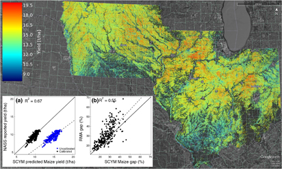
Figure 1 Map of average SCYM maize yield estimates in the study region, 2000–2015. Inset (a) compares average county maize yields with USDA reports. 'Uncalibrated' show raw SCYM estimates averaged over 2000–2015, while 'calibrated' show estimates corrected using the best-fit line (dashed). Solid line shows 1:1. Inset (b) compares maize 'yield gaps' estimated from calibrated SCYM estimates and a database of farmer-reported yields from RMA. Here 'yield gaps' are defined as the difference between the 95th percentile and mean of yields across fields within a county. These values are computed for each year with overlap between the two datasets (2000–2012), with the average across years shown in the plot.
Download figure:
Standard image High-resolution image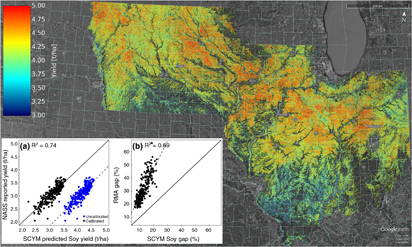
Figure 2 Map of average SCYM soybean yield estimates in the study region, 2000–2015. Inset (a) compares average county soybean yields with USDA reports. 'Uncalibrated' show raw SCYM estimates averaged over 2000–2015, while 'calibrated' show estimates corrected using the best-fit line (dashed). Solid line shows 1:1. Inset (b) compares soybean 'yield gaps' estimated from calibrated SCYM estimates and a database of farmer-reported yields from RMA. Here 'yield gaps' are defined as the difference between the 95th percentile and mean of yields across fields within a county. These values are computed for each year with overlap between the two datasets (2000–2012), with the average across years shown in the plot.
Download figure:
Standard image High-resolution imageThe SCYM estimates also are able to capture spatial differences in the within-county yield heterogeneity evident in the RMA data (figures 1(c) and 2(c)). For maize, the measures are highly correlated with RMA (R2 = 0.55) and fall close to the 1:1 line. For soybean, the correlation is higher (R2 = 0.66) but SCYM tends to understate yield heterogeneity relative to RMA. Overall, the RMA data indicate that SCYM estimates of heterogeneity predominantly reflect true yield heterogeneity rather than noise, and can discriminate between counties with low vs. high heterogeneity. The satellite-based measures of heterogeneity have the added advantages that they are (i) available for a much larger sample of fields than the public RMA data, (ii) available for more recent years, and (iii) allow inspection of within-field heterogeneity, since a typical field contains hundreds of 30 × 30 m pixels.
Magnitude of between and within-field yield heterogeneity
YH0 and YHIF calculations for a single county are illustrated in figure 3, along with maps of average YHO and YHIF for 2000–2015 for all counties. These maps indicate four notable features. First, YHO is typically below 40% for both crops, supporting the notion of relatively modest yield gaps in this region (Grassini et al 2015, Fischer et al 2014, Lobell et al 2009, van Wart et al 2013). Second, soy YH is generally smaller than maize YH, with a production-weighted average YHO of 27% across the region, compared to 35% for maize. This suggests that soybean yields are even closer to their yield potential than maize in this region, as argued previously (Fischer et al 2014), although an important caveat is that SCYM estimates of heterogeneity appear more biased downward for soybean than maize (figure 3(c)).
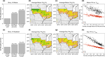
Figure 3 (a) Example of calculation of maize YHIF and YHO for Story County, IA. (b) and (c) Maps of average YHO and YHIF for 2000–2015 (note different legends). (d) Comparison of YH measures vs. average yields. (e)–(h) Same as (a)–(d) but for soybean.
Download figure:
Standard image High-resolution imageThird, YHIF is commonly half or more of YHO. This finding suggests that conditions which vary within fields, namely soil conditions and landscape position, are relatively important drivers of yield variability, above and beyond factors that only vary across fields, such as farm ownership or management. Moreover, it emphasizes the importance of fine-scale heterogeneity in these soil and landscape factors, as argued by (Brandes et al 2016), which limits the utility of coarse resolution soil maps.
Fourth, YHO is significantly larger in the lower yielding counties that span the southern edge of all three states (figures 3(d) and (h)). These counties lie below the regions of major glacial till and are characterized by shallower and more heterogeneous soil conditions that are less favorable to crop growth. The steep increase in YHO for these counties again indicates the importance of soil conditions in driving YH in the region. A negative relationship between percentage yield gaps and average yields has also been recently observed in Australian wheat systems (Gobbett et al 2016), though in that study the absolute yield gaps (in t ha−1) were larger in higher yielding areas. Here, we find that both relative and absolute yield gaps are highest in lower yielding counties.
Trends of between and within-field yield heterogeneity
Over the sixteen year record of Landsat data used in this study, both YHO and YHIF exhibit widespread increases (figure 4). Nearly every county has experienced an increase in maize YHO and YHIF, sometimes with as much as a 15 percentage point increase in the measure of heterogeneity over the study period. Changes in YH for soybean are more mixed than for maize, with the majority of counties still showing increases but many showing decreases.

Figure 4 (a) Maize YHIF and YHO for Story County, IA over the study period, with best-fit linear trends (dashed lines). (b) and (c) Maps of trends in YHO and YHIF. (d)–(f) Same as (a)–(c) but for soybean.
Download figure:
Standard image High-resolution imageAlthough figure 4 displays trends in two specific measures of heterogeneity (YHO and YHIF), the overall increase in heterogeneity is also readily apparent when examining the full yield distributions over time. For example, figure 5 displays the histogram of yields for the entire study area for the first three and last three years of the study for each crop. For maize, there is a clear rightward shift in the upper half of the distribution, but little change at the lower end. This results in a clear widening of the distribution, indicative of greater yield heterogeneity. This figure also indicates that overall yield gains have largely resulted from increases in yields at the upper end of the distribution, rather than from a uniform shift of the distribution to the right. Soybeans show a much less dramatic shift in the yield distribution.
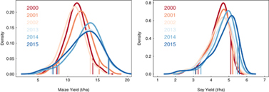
Figure 5 Histograms of maize and soybean yields across the study region for the first three and last three years of the study period. Maize yields exhibit a widening of the yield distribution, consistent with the county trends shown in figure 4, whereas soybeans show mainly a (small) shift in the distribution to the right but little widening. Vertical lines indicate the 5th and 95th percentiles of the distribution in each year.
Download figure:
Standard image High-resolution imageMany factors cause yields to vary within and between fields within a county, and increases in heterogeneity indicate that one or more of these factors have been growing in importance over time. To explore the importance of one factor for which widespread (albeit imperfect) data exist, we calculated yields and yield changes as a function of soil properties reported in the gridded SSURGO database (National Resource Conservation Service 2014). The gridded SSURGO data is provided at 10 m, and therefore we first aggregated it to the 30 m resolution of the yield estimates. Two key soil attributes were considered: USDA's national commodity crop productivity index (NCCPI), an integrated measure of land suitability, and total root zone available water storage (RZNAWS). For each soil attribute, we computed the distribution of values across the study region and identified 'favorable' and 'unfavorable' soils as those with values above the 80th percentile or below the 20th percentile. For NCCPI, the values identified were 85 and 48, whereas for RZNAWS the values were 293 and 154 mm. (The value of 154 mm is nearly identical to the 152 mm (6 inches) threshold used to define 'droughty' soils by the USDA (National Resource Conservation Service 2014).)
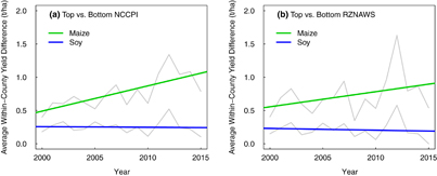
Using these thresholds, for each county we calculate the yield differences between pixels with 'favorable' and 'unfavorable' soils, and the change in these differences over time. Although the gSSURGO data are far from perfect, for instance with obvious discontinuities at county borders, any errors would cause us to be overly conservative in assessing yield impacts of soil factors as long as the errors were uncorrelated with our yield estimates. The average within-county yield difference was positive in all years for both maize and soybean (figure 6), indicating unsurprisingly that yields are higher on the better soils within each county. More surprising, we find that within-county differences between high and low NCCPI have been steadily growing for maize (p < 0.01), but not for soybean. For maize, the average yield difference between pixels in the top and bottom 20% of NCCPI more than doubled from roughly 0.5 ton ha−1 in 2000 to over 1.0 ton ha−1 by 2015. Results were similar for RZNAWS, though less significant for maize (p = .17).
Figure 6 (a) Average within-county yield difference between pixels with high and low NCCPI values for each year. Gray lines show values for individual years and colored lines indicate linear trends. (b) same as (a) but for RZNAWS (root zone available water storage).
Download figure:
Standard image High-resolution image
What factors are driving increased yield heterogeneity?
Any proposed explanation for the observed increase in yield heterogeneity should be consistent with the above observations that (i) increases are evident both within and between fields, (ii) the increases are much more apparent in maize than in soybean and (iii) maize yield differences between 'poor' and 'good' soils appear to be growing over time. For example, we do not consider errors in the SCYM estimates as a plausible explanation, since any artifacts that are changing over time (e.g. from scan-line gaps in Landsat 7 imagery) should be seen equally regardless of crop or soil type. Two explanations seem particularly likely, though it is difficult to determine how much each contribute to the overall trends.
First, a major trend in recent years has been the adoption of variable rate technologies (VRT), particularly since 2010 (Erickson and Widmar 2015). These techniques attempt to precisely distribute inputs such as fertilizers and seeds throughout a field, rather than applying them uniformly. VRTs are often input-neutral, in that the total amount of inputs for a field changes very little from prior practices, but with some parts of the fields receiving much more inputs than other parts. If better parts of a field are more responsive to inputs, farmers adopting VRT will tend to increase inputs to the better parts of their fields and reduce inputs in other parts. In this way, adoption of VRT would tend to exacerbate yield gradients within fields.
A second important trend that would lead to higher heterogeneity is the continued increase in sowing density. A significant driver of yield gains in maize over the past decades has been the combination of stress-tolerant hybrids and denser sowing (Tollenaar and Wu 1999, Duvick 2005), and high sowing density is known to be most effective in raising yields under conditions of ample soil water and nutrients and favorable (cooler) temperatures (Ruffo et al 2015, Lobell et al 2014, Duvick 2005). Thus, even if this management change was applied uniformly by farmers, it would be expected to result in increased yield heterogeneity.
A third potential explanation for rising heterogeneity could be that certain weather conditions that lead to more heterogeneity have been changing over time. To evaluate this explanation, we computed for each county the correlation between YHO and two weather measures known to be important for crop yields in the region: total precipitation for June-August (RAIN), and average daytime vapor pressure deficit during the key month of July (VPD). Conditions of high VPD and/or low RAIN are known to stress crops and reduce yields (Lobell et al 2014). We find that these conditions are also likely to increase YHO in most counties (figure S3), with generally positive correlations between YHO and VPD, and negative correlations between YHO and RAIN. However, we also find that trends in these conditions were typically small over the study period, and as a result calculating trends in YHO while simultaneously accounting for both VPD and RAIN has very little effect on the estimated trends in YHO (figure S3). Thus, we conclude that weather trends have been far less important than management changes in driving increased heterogeneity.
The data available for the current study do not allow us to discern the relative contribution of VRT and sowing density to heterogeneity increases. Both of these explanations are consistent with the criteria laid out, as they both would affect heterogeneity within fields, disproportionately affect better soils, and affect maize more than soybean (Adoption of VRT is not reported by crop, but is anecdotally applied more to maize than soybean. Soybean has not experienced the same change in sowing density as maize (Lobell et al 2014).) Alternative explanations, such as changes in management driven by crop prices or weed resistance, appear less consistent with the criteria, but cannot be ruled out with current datasets.
In either case, the growing difference between yields on good and poor soils (figure 6) indicates that maize yield gains since 2000 are coming disproportionately from better soils. This trend of 'the rich getting richer' suggests that renewed effort is needed for raising yields in more marginal conditions. At the same time, the large and rising heterogeneity within fields also indicates that the incentives for precision agriculture (including VRTs as well as conversion of parts of fields to perennials (Brandes et al 2016)) is growing, because the economic and environmental cost of managing the entire field as a single unit is growing.
Conclusions
The combination of public Landsat imagery, cloud computing platforms such as Google Earth Engine, and robust algorithms such as SCYM present new opportunities for studying agricultural landscapes. Whereas prior work has had to rely on county-level aggregates or occasional datasets on field aggregates, it is now possible to examine 16 years of sub-field heterogeneity across the Corn Belt. The data used in this study were derived entirely from public sources, and the approach could be readily repeated in other regions. This is particularly promising in light of the recent growth of the microsatellite industry, which provides data capable of resolving fields in the smallholder systems that predominate in much of the world.
Among the insights gained from this new dataset, two stand out as particularly noteworthy. One is that a substantial fraction of overall yield heterogeneity derives from within-field variation. This result underscores the importance of soil constraints in this region, presumably because management skill or incentives are not very heterogeneous across farms. Second, the results indicate a significant increase in maize YH in recent decades, with larger YH both within and between fields. This trend reflects a preferential rate of yield progress in favorable soil conditions, which likely results both from the adoption of variable rate technologies and the disproportionate benefit of denser sowing on better soils. Whether yield progress on better soils can continue to sustain aggregate yield growth in the region (figure S1) remains to be seen. At the same time, the rising benefit of employing tools of precision agriculture combined with their declining cost suggests the possibility of rapid improvements in reducing mis-applications of inputs and associated runoff and leaching of nutrients from agriculture.
This work was supported by a Terman Fellowship and Google Earth Engine Research Award to DBL and the Fink Foundation. We thank Evan Lyons for help processing the gSSURGO data, Marshall Burke, Ken Cassman, Tony Fischer, Christopher Seifert and two anonymous reviewers for helpful comments on the manuscript, and the Google Earth Engine team for providing technical support and computing resources. The datasets developed in this study will be made available upon request via the Earth Engine platform.