

Abstract
A quantification of present and future mean annual losses due to extreme coastal events can be crucial for adequate decision making on adaptation to climate change in coastal areas around the globe. However, this approach is limited when uncertainty needs to be accounted for. In this paper, we assess coastal flood risk from sea-level rise and extreme events in 120 major cities around the world using an alternative stochastic approach that accounts for uncertainty. Probability distributions of future relative (local) sea-level rise have been used for each city, under three IPPC emission scenarios, RCP 2.6, 4.5 and 8.5. The approach allows a continuous stochastic function to be built to assess yearly evolution of damages from 2030 to 2100. Additionally, we present two risk measures that put low-probability, high-damage events in the spotlight: the Value at Risk (VaR) and the Expected Shortfall (ES), which enable the damages to be estimated when a certain risk level is exceeded. This level of acceptable risk can be defined involving different stakeholders to guide progressive adaptation strategies. The method presented here is new in the field of economics of adaptation and offers a much broader picture of the challenges related to dealing with climate impacts. Furthermore, it can be applied to assess not only adaptation needs but also to put adaptation into a timeframe in each city.
Export citation and abstract BibTeX RIS

Original content from this work may be used under the terms of the Creative Commons Attribution 3.0 licence. Any further distribution of this work must maintain attribution to the author(s) and the title of the work, journal citation and DOI.
1. Introduction
Assessing expected damage costs of local sea-level rise (LSLR) in coastal cities provides key input to help decision makers decide on the best ways to cope with climate change in many urban areas of the world. The traditional approach to assessing these costs is based on measuring annual average losses of extreme events of different return periods in a deterministic way. However, there is an increasing need for alternative economic decision support tools that better account for climate change uncertainty (Watkiss et al 2015). Recent studies have proposed a new paradigm to develop robust adaptation planning in a dynamic framework (Hallegatte 2009) as an effective way of dealing with uncertainty. In addition, the concept of 'adaptation pathways' has also been proposed to guide decision making in a context of deep uncertainty. The latter presents adaptation decision-making as a sequence of possible actions over time, which allows for monitoring, revision and adjustment in the light of new information (Haasnoot et al 2011, 2013). A good example of dynamic robust approaches can be found in Ranger et al (2013) for the Thames 2100 project design.
A recent editorial in Nature Climate Change reminded us that special attention should be paid to socio-economic impacts of significant but less likely climatic events (Editorial 2016). These low-probability, high-damage impacts have been repeatedly discussed earlier in climate change economics literature (Weitzman 2007, 2009, Nordhaus 2011, Weitzman 2013) and are very important due to the huge magnitude of their potential damage (Pindyck 2011). Hinkel et al (2015) also argue in favor of providing estimates of low confidence situations as they are very much needed for risk-adverse decision making, especially considering that IPCC scenarios focus on the central distribution rather than the high-risk tail and the presence of deep uncertainty. Central distributions are not adequate to guide decisions of coastal managers as population in coastal zones usually show a strong aversion to major floods (Hinkel et al 2015).
This paper proposes a risk measure approach that can effectively support adaptation planning processes to help to deal with uncertainty through many stochastic models of LSLR that generate the corresponding stochastic model of damages, using local damage functions. Based on the local probability distributions of damages obtained stochastically, we estimate two risk measures that are widely used in the field of finance economics with regard to the probability of rare, adverse events from which one wishes to be protected.
Other studies have developed frameworks to account for uncertainty in relation to the expected losses due to sea-level rise and coastal extreme events. For instance, Boettle et al (2013) used extreme value theory with the block-maxima approach for two Danish cities, Copenhagen and Kalundborg. They analyze the expected damage and the standard deviation as a function of varying location and scale parameters of the generalized extreme value distribution (GEV). Boettle et al (2016) likewise used a Generalized Pareto Distribution (GPD) to assess the impact of sea-level rise as well as potential protection measures on the flood damage for the previous two cities, Copenhagen and Kalundborg. They assumed that a rise in mean levels results in a shift of today's sea level distribution.
The approach proposed in this paper introduces several innovations compared to previous work: first, it is applied to many coastal cities (as many as 120) using LSLR estimations; second, our model is compatible with the IPCC emission scenarios (RCP2.6, 4.5 and 8.5); third, it allows for a yearly evolution of damages from 2030 to 2100 as it uses a continuous stochastic diffusion process; and fourth, it provides an estimation of two risk measures that puts low-probability, high-damage events in the spotlight, filling the information gap regarding the high-risk tail identified by Hinkel et al (2015) in a context of coastal decision-making. Furthermore, these risk measures as well as the stochastic modelling are necessary steps for the application of other robust methodologies such as Real Option Analysis.
To the best of our knowledge, this approach has not been previously used for assessing climate risk, and more precisely, the impacts of LSLR and coastal extremes. The method can guide the adaptation pathways approach offering detailed information coherent with different levels of acceptable risk.
2. A stochastic approach for modelling LSLR under uncertainty
2.1. Data on relative sea-level rise at the local scale
Regionalized data on sea-level rise under the latest IPCC emission scenarios have been published in recent years. For example, Grinsted et al (2015) estimated the probability distributions of LSLR for several cities in Northern Europe under RCP8.5. Kopp et al (2014) obtained LSLR projections for a large number of locations and three RCP emission scenarios, RCP2.6, 4.5 and 8.5. The latter combined expert elicitation with AR5 projections in order to estimate the contribution of the Greenland and Antarctica Ice Sheets to sea-level rise, while the results from Grinsted et al (2015) in relation to this component are based solely on expert elicitation. All these reasons explain why the data from Kopp et al (2014) are more suitable for our analysis.
A comprehensive dataset of local sea-level rise was developed by Kopp et al (2014) for several hundred locations around the world. These local estimates represent relative changes in sea-level, i.e. the net difference between the surface of the ocean and the continent (Lambeck et al 2010). Kopp et al (2014) have accounted for the following components of LSLR: (i) changes in ocean dynamics; (ii) static equilibrium effects; (iii) glacial isostatic adjustments; (iv) other local non-climatic drivers, such as groundwater depletion, sediment compaction or tectonic processes. Differences in LSLR compared to global changes can be significant, so working with regionalized data is critical. Kopp et al (2014) provide estimates of medians and some percentiles, which allow us to calibrate the stochastic model and generate a full distribution of probabilities for each location, in order to later analyze low-probability, high-impact tail events.
2.2. Stochastic model and risk measures
Using the LSLR data from Kopp et al (2014), we have obtained each of the LSLR probability distributions from 2030 to 2100 as a continuous function for any of the 120 coastal mega cities2 in the study under three IPCC emission scenarios (RCP2.6, 4.5 and 8.5). This was performed using a continuous stochastic Geometric Brownian Motion (GBM) diffusion model, a very common model defined as 'a stochastic process often assumed for assets where the logarithm of the underlying variable follows a generalized Wiener process' (Hull 2012). This is very suitable to model LSLR as it can be very well calibrated for the information provided by Kopp et al (2014).
The GBM model parameters (drift and volatility) for LSLR were calibrated using the data from Kopp et al (2014) for three of the latest IPCC emission scenarios or Representative Concentration Pathways, (RCP 2.6, 4.5 and 8.5). This allows a LSLR distribution function that is log-normal at all times. The expected LSLR drift is obtained by minimizing the sum of the square of the differences with the theoretical median values (2030, 2050 and 2100). The volatility is calculated with the 95th percentile using the log-normal distribution proprieties. In this case, we have information for 120 cities in the world for the three different IPCC scenarios. This is equivalent to 360 stochastic models with different parameters (drift and volatility). As a result of these calculations, we finally obtain a damage distribution for each city and each IPCC scenario every 5 years from 2030 to 2100. Figure 1 below shows the full probability distribution of damages for New Orleans in 2050 and under three emission scenarios.
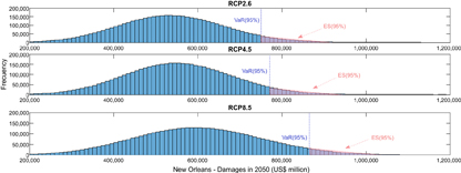
Figure 1 Probability distribution of damages in 2050 for New Orleans, under RCP2.6, 4.5 and 8.5.
Download figure:
Standard image High-resolution imageIn addition to this, the damage distribution enables us to calculate two measures of risk: the Expected Shortfall (ES) and Value at Risk (VaR)3. The VaR(1-α) of a portfolio at the confidence level α is the value at which the probability of obtaining higher values is exactly 1-α. In the case considered here, it represents the level of damage caused by SLR for which the probability of a higher damage is α. Therefore, the VaR assesses the maximum losses that could occur with a given confidence level for a given time frame or the level above which we enter a certain 'low-probability, high-impact zone' on the probability distribution. In the present study, the confidence level was set at 95% and the time t, is measured in years but any other α could be used. (See figure 1).
Expected Shortfall (ES) is here the expected value when the damage is greater than VaR(1 − α) or, in other words, the mean value in the 'low-probability, high-impact zone'. Note that ES is a better risk measure as it gives more information on expected losses in less favorable situations than just a level of a critical threshold represented by VaR. Additionally, ES provides optimization short-cuts which, through linear programming techniques, make many large-scale calculations practical that would otherwise be out of reach.
These risk measures can be calculated for bigger or smaller zones, i.e. for greater or smaller percentiles, to test the sensitivity of results to uncertainty in the tails (the so-called tail of the tails). In our example, we are looking at 95 percentiles but note that ES (95%) additionally provides significant information with regards to what is happening within the high-risk tail.
In the risk calculation process, we used Monte Carlo to simulate 5,000,000 SLR values for each scenario and time t.
2.3. The damage function
We estimate expected economic losses of LSLR (in monetary terms) for each city using site-specific damage functions. These functions are constructed as follows: first, LSLR at time t in each city and for each scenario is estimated using the stochastic GBM model as described in section 2.2; second, we use information on the damage functions for each city based on population, economic development and assets at risk from Hallegatte et al (2013); finally, we estimate the distribution of different extreme flood levels in each city combining the information from our stochastic model together with the damage function from Hallegatte et al (2013). As our LSLR estimates are stochastic, when we apply this function to the damage function from Hallegate, we obtain a probability distribution of the damages (in monetary terms). Note that the damage function from Hallegatte et al (2013) accounts for the effect of SLR and coastal extreme events, and consequently the damages on our study correspond to the combination of both effects. This implies that our results are subject to the limitations and uncertainties existing in the damage function by Hallegatte et al (2013).
Specific LSLR in each city, emission scenario and time t can lead to some particular damage costs. As a consequence of this process, we are taking uncertainty into consideration through the stochastic modelling offering a much more detailed and realistic picture of the risks. This information is especially useful for risk averse decision making. Note that the model presented here can be adapted to incorporate new information when this becomes available. In this application we are limited by the lack of homogeneous data on damage functions, but the model could be updated as better data becomes available and results re-estimated to offer a broader and more reliable picture.
Once the damage distribution has been generated, the 95% percentile VaR (95%) and ES (95%) can be calculated. In this case, we have 250,000 values for the damages of the most unfavorable situations, which enable us to obtain highly accurate values of ES (95%). Remember that VaR (95%) is the value of the loss corresponding to the damage function in the 95% percentile or the level at which we enter the 'low-probability, high-impact' zone while ES (95%) refers to the mean expected loss in that same zone or when the value VaR is exceeded. In this case we are considering α = 5%, but the model can be processed for any value of α.
3. Defining risk thresholds: towards progressive adaptation strategies
At this stage, a certain level of risk or critical-risk threshold based in a percentage loss equivalent to each city's GDP in 2030 can be defined, even though any other reference could be easily applied. In our paper, and for illustration purposes, the levels assumed are 1% and 2% of each city's GDP in 2030. However, these thresholds could be defined in a real policy-making context with the participation of policy makers, risk managers and other stakeholders and be solely based on their risk aversion.
This critical risk threshold can be calculated for any given year as we have estimated a continuous damage function. Consequently, we can obtain the year when each city is expected to have adaptation measures fully operative according to the actual information. This analysis can be repeated later in time when new information becomes available. Of course, as many sources of uncertainty may exist in climate related projections, one could argue in favor of undertaking sensitivity analysis with a range of values for acceptable levels of risk and/or percentiles to illustrate the variation of the years in which adaptation measures should be ready to be used. This is performed for each city and emission scenario looking for the moment in time when ES (1 − α), in our case 1 − α = 95% interval, so the maximum acceptable damage (1% and 2% of each city's GDP in 2030) is only exceeded in 5% of cases.
One of the strengths of our method is that it helps to put adaptation into a timeframe using a standard and easy to comprehend indicator such as GDP to define acceptable level of risk. Policy makers, as well as other stakeholders, that regularly make budgetary decisions, can well understand the size of the damages in terms of GDP losses.
4. Findings and results
Table 1 shows the expected mean annual economic loss estimates for the top 20 cities using the stochastic model. In this model, damage costs vary greatly depending on the city and IPCC scenario considered. Most of the cities in the ranking are Asian cities. Note however that four US cities are in the top 20 of those most affected by coastal extreme events: New Orleans, which leads the ranking, New York, Boston and Houston.
Table 1. Cities ranked by expected annual average losses (AAL) in 2050.
| AAL (US$ million) | |||||
|---|---|---|---|---|---|
| ID | City | Country | RCP2.6 | RCP4.5 | RCP8.5 |
| 1 | New Orleans | USA | 539,200 | 554,973 | 603,350 |
| 2 | Guangzhou Guangdong | China | 346,032 | 375,053 | 456,394 |
| 3 | Bangkok | Thailand | 323,092 | 334,940 | 364,059 |
| 4 | Calcutta | India | 198,283 | 210,923 | 235,809 |
| 5 | Osaka-Kobe | Japan | 180,943 | 187,319 | 213,040 |
| 6 | Mumbai | India | 121,190 | 132,452 | 189,435 |
| 7 | Alexandria | Egypt | 67,683 | 66,586 | 84,194 |
| 8 | Shangai | China | 62,792 | 71,576 | 90,486 |
| 9 | Tokyo | Japan | 59,531 | 67,795 | 87,524 |
| 10 | Tianjin | China | 56,895 | 64,084 | 77,751 |
| 11 | Guayaquil | Ecuador | 37,635 | 43,459 | 58,784 |
| 12 | Zhanjiang | China | 29,990 | 32,569 | 37,833 |
| 13 | Shenzen | China | 26,850 | 31,261 | 46,543 |
| 14 | Surat | India | 26,445 | 27,957 | 33,221 |
| 15 | New York | USA | 25,743 | 29,389 | 36,509 |
| 16 | Ho Chi Minh City | China | 24,349 | 27,544 | 35,487 |
| 17 | Hai Phòng | Vietnam | 23,077 | 27,478 | 39,758 |
| 18 | Boston | USA | 23,059 | 26,746 | 34,725 |
| 19 | Fukuoka-Kitakyushu | Japan | 22,334 | 23,995 | 28,496 |
| 20 | Houston | USA | 18,573 | 19,225 | 21,500 |
The mean losses for the 120 cities by 2050 range from US$2,478 billion to US$3,162 billion (table A1). These results are much higher than previous values from Hallegatte et al (2013)4. The main reason for this is that the study by Kopp et al (2014) forecasts much greater (in some cases up to 3 times higher) sea-level rise than the former.
If we now consider the expected damages in the 'low-probability, high-impact zone' (see table 2), the losses in 2050 can be up to 746% higher and at least 139% higher than the mean expected values. Results for all 120 cities are available in table A2.
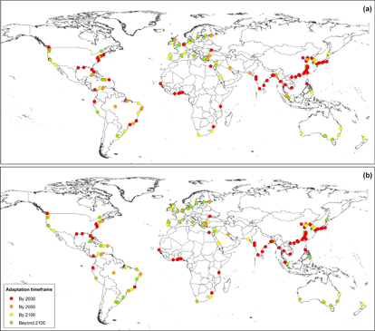
Understanding the magnitude of the risk that arise in the upper tail of the distribution is very important for coastal managers. As stated earlier, the methodology presented here can also shed some light into the right timing when protection measures should be in place to safeguard a city5. This is shown in figure 2 (and table A3 for all cities and RCPs), where we present the year in which defenses should be already in place depending on two levels of acceptable risk (1% or 2% of each cities' GDP) for RCP 4.5 scenario. In both cases, the lower and higher risk aversion thresholds, all the cities in the top 20 ranking in table 2 should have undertaken adaptation before 2030 in all three IPCC scenarios (see table A3). The figures show some modest changes in the colors for cities, representing changes in the timing for adaptation for long time periods, depending on the level of acceptable risk. More detailed information for each city, RCP and level of acceptable risk can be found in table A3. Note that the levels of acceptable risk in this paper have been chosen for illustrative purposes and do not imply any normative statement. In many cases, especially in developed and rich countries, these levels of risk may imply significant damages worth millions of US$ that could be considered unacceptable losses. The method presented here allows for any given level of acceptable risk to be similarly calculated6.
Figure 2 Maps representing the timeframe for adaptation for each city under RCP4.5. The risk threshold is 1% of each city's GDP in figure 2(a) and 2% in figure 2(b).
Download figure:
Standard image High-resolution image
Table 2. Ranking of cities considering the 95 percentiles of expected shortfall (ES) and value at risk (VaR) by 2050, under RCP2.6.
| RCP2.6 | RCP4.5 | RCP8.5 | ||||||
|---|---|---|---|---|---|---|---|---|
| ID | City | Country | VaR (95%) | ES (95%) | VaR (95%) | ES (95%) | VaR (95%) | ES (95%) |
| 1 | Guangzhou | China | 804,357 | 966,539 | 822,687 | 976,248 | 911,470 | 1,061,446 |
| 2 | New Orleans | USA | 751,872 | 808,642 | 769,535 | 826,795 | 863,879 | 934,071 |
| 3 | Bangkok | Thailand | 423,428 | 449,846 | 439,551 | 467,128 | 489,965 | 523,386 |
| 4 | Mumbai | India | 290,058 | 348,064 | 298,988 | 354,191 | 377,980 | 438,366 |
| 5 | Calcutta | India | 298,250 | 325,955 | 313,204 | 341,546 | 353,424 | 386,322 |
| 6 | Osaka-Kobe | Japan | 272,018 | 297,271 | 280,101 | 305,837 | 320,692 | 350,882 |
| 7 | Alexandria | Egypt | 223,444 | 283,555 | 162,098 | 192,951 | 203,389 | 241,864 |
| 8 | Tianjin | China | 135,914 | 162,009 | 138,539 | 162,128 | 155,847 | 180,091 |
| 9 | Shangai | China | 138,808 | 161,599 | 149,796 | 173,014 | 177,597 | 203,424 |
| 10 | Guayaquil | Ecuador | 114,619 | 147,096 | 123,702 | 155,097 | 150,777 | 183,419 |
| 11 | Tokyo | Japan | 127,451 | 146,901 | 133,747 | 152,672 | 158,233 | 179,323 |
| 12 | Shenzen | China | 96,090 | 127,400 | 101,314 | 129,923 | 127,754 | 156,933 |
| 13 | Hai Phòng | Vietnam | 73,554 | 91,314 | 79,817 | 97,367 | 99,584 | 118,651 |
| 14 | Nagoya | Japan | 56,589 | 74,304 | 57,953 | 71,874 | 66,364 | 78,311 |
| 15 | Ho Chi Minh City | China | 61,211 | 73,192 | 64,247 | 75,794 | 75,386 | 87,645 |
| 16 | Boston | USA | 56,846 | 67,840 | 60,539 | 71,179 | 73,288 | 85,337 |
| 17 | Zhanjiang | China | 57,248 | 65,489 | 59,967 | 68,183 | 66,930 | 75,619 |
| 18 | New York | USA | 55,732 | 65,136 | 60,510 | 70,117 | 71,350 | 82,059 |
| 19 | Surat | India | 48,483 | 54,989 | 49,609 | 55,940 | 56,626 | 63,469 |
| 20 | Miami | USA | 40,399 | 47,567 | 42,721 | 49,724 | 50,547 | 58,333 |
It is important to note that having information on the timeline in which the adaptation measure should be operative is an expectation today that can guide adaptation pathways. This will likely change as time passes, and two possibilities arise:
- There is not (or just about) enough time to build the adaptation measure or defense before the critical threshold is exceeded. In such a case the protection should start to be built urgently, and decide whether this should be flexible or not.
- If there is enough time to build the defense before the critical threshold is exceeded, then it may be reasonable to wait for few years to make a decision and produce new calculations when the new information becomes available. This is a very good example of flexible or progressive adaptation policy.
Previous works have also suggested the use of adaptation options that can be changed or adjusted in time as more information becomes available (see, for example, Kwakkel et al 2015). Building up flexibility in decision-making for planning adaptation infrastructures is a great challenge, but it can be achieved through this method, which can be updated as soon as the available information improves (IPCC 2014). In this line, Haigh et al (2014) state that higher rates of global sea level rise will likely be detectable by 2020. The model could be updated when this information becomes available.
Conclusions
The method presented here for modelling LSLR with a stochastic diffusion model is a novelty that allows constructing a continuous function of the probability distribution of flood damages (in monetary units) in each given city. This is a very important piece of information for coastal risk management as it allows for a more detailed risk analysis looking at low-probability, high-impact events, the so-called high-risk tail. Many authors have argued before about the pertinence of such information to guide adaptation policies (Hinkel et al 2015, Editorial 2016).
Incorporating stochasticity to the uncertainty analysis also allows us to calculate risk measures such as VaR and the more suitable measurement of risk ES. The latter provides a great deal of information on what is happening within the high-risk tail while it also allows for time-framing adaptation policies, as shown in this paper. This framing will be based in a certain level of acceptable risk that can be tailored to each city based on, for example, the result of participatory consultations with informed risk managers, decision makers and other stakeholders. This is a very important attribute of the approach presented here that is based on rigorous and highly quantitative methods, while, at the same time, it can incorporate measures of risk aversion defined by stakeholders. Another advantage is that results can be easily explained and communicated.
We have argued that these calculations allow decisions to be made as to whether a flood defense is expected to be urgent in any given city or, on the contrary, the decision to have it operative can be postponed until more reliable information is available. This is the kind of policy questions that decision makers need to answer when designing adaptation pathways.
Finally, another co-benefit of this model is that it permits other types of robust and sophisticated economic approaches (such as Real Options analysis) to be undertaken to assess the value of postponing an investment decision or deciding to invest in a flexible defense that might admit a greater degree of protection in the future, if this is required. Additionally, our model allows sensitivity analysis to be developed, accounting for several parameters, such as drift, volatility and even the damage function. An example of a sensitivity analysis can be found in the supplementary material (stacks.iop.org/ERL/12/014017/mmedia).
The authors acknowledge funding from the European Union's Seventh Framework Programme for research, technological development and demonstration under grant agreement no 603906, Project: ECONADAPT and Horizon 2020 Project RESIN (grant agreement no. H2020-DRS-9-2014). LMA and IG are grateful for the financial support received from the Basque Government for support via project GIC12/177-IT-399-13. LMA also thanks financial support from the Spanish Ministry of Science and Innovation (ECO2015-68023).
Author contribution
All three authors participated in the design of the research question and methodological setting. LMA was in charge of the programming and calculations. All three contributed to the analysis and writing-up.
Conflict of interest
The authors declare that they hold no competing financial or non-financial interests.
Footnotes
- 2
- 3
A detailed explanation of risk measures can be found in Artzner et al (1999).
- 4
Results for all cities are also presented in the annex in table A1.
- 5
Of course, an adaptation planning process should account for the time lag that exists between the decision to adapt and when the protection is actually in place (Hinkel et al 2015).
- 6
Calculations for acceptable levels of risk of 0.1% and 0.5% of GDP are available upon request.