

Abstract
Crop yields must increase substantially to meet the increasing demands for agricultural products. Crop yield increases are particularly important for Russia because low crop yields prevail across Russia's widespread and fertile land resources. However, reliable data are lacking regarding the spatial distribution of potential yields in Russia, which can be used to determine yield gaps. We used a crop growth model to determine the yield potentials and yield gaps of winter and spring wheat at the provincial level across European Russia. We modeled the annual yield potentials from 1995 to 2006 with optimal nitrogen supplies for both rainfed and irrigated conditions. Overall, the results suggest yield gaps of 1.51–2.10 t ha−1, or 44–52% of the yield potential under rainfed conditions. Under irrigated conditions, yield gaps of 3.14–3.30 t ha−1, or 62–63% of the yield potential, were observed. However, recurring droughts cause large fluctuations in yield potentials under rainfed conditions, even when the nitrogen supply is optimal, particularly in the highly fertile black soil areas of southern European Russia. The highest yield gaps (up to 4 t ha−1) under irrigated conditions were detected in the steppe areas in southeastern European Russia along the border of Kazakhstan. Improving the nutrient and water supply and using crop breeds that are adapted to the frequent drought conditions are important for reducing yield gaps in European Russia. Our regional assessment helps inform policy and agricultural investors and prioritize research that aims to increase crop production in this important region for global agricultural markets.
Export citation and abstract BibTeX RIS

Content from this work may be used under the terms of the Creative Commons Attribution 3.0 licence. Any further distribution of this work must maintain attribution to the author(s) and the title of the work, journal citation and DOI.
1. Introduction
Global agricultural production must increase substantially to satisfy the growing demand for agricultural products that has resulted from population growth, higher-calorie diets, and the use of land-based resources for biofuel production (Godfray et al 2010). Two options are available for increasing agricultural production. The first option is to increase the area of cultivated land. However, further expansion carries considerable environmental costs (Foley et al 2005, Lambin and Meyfroidt 2011). The second option is to enhance productivity on existing agricultural lands. Higher yields may prevent the conversion of non-agricultural lands into agricultural lands because more output would be obtained from the existing agricultural land (Green et al 2005, Rudel et al 2009). Thus, increased crop yields will be important for satisfying the growing demands for food, feed, fuel, and fiber while minimizing adverse environmental effects (Mueller et al 2012).
However, current yield improvements may occur too slowly to meet the increasing demands for agricultural products (Ray et al 2013). Moreover, the potential for improving crop yields varies widely around the world, and large yield gaps (i.e., differences between potential and actual yields) are common. For example, the yield gaps are generally large in developing and transitional countries, in which substantial limitations in agricultural management, infrastructure, education, and agricultural policies often impede increases in land productivity (Neumann et al 2010, Tilman et al 2011). Conversely, many developed countries have already crop yields that are close to its yield potentials, and the costs of additional yield increases could outweigh the economic benefits (Lobell et al 2009). Better data and knowledge regarding the sizes, spatial distributions, and determinants of yield gaps could be used to target policies and management practices that increase crop productivity.
Crop growth models can estimate potential yields by simulating the optimal management conditions that ensure crop growth under conditions with no stress from weeds, pests, and diseases and with sufficient available nutrient content and water (Evans and Fischer 1999). Under such optimal management conditions, the yield potential becomes a function of the prevailing climate, biophysical conditions, and cultivars. Consequently, the effects of crop management on yields can be tested (Lobell et al 2009).
Crop growth models can accurately estimate yield potentials at small spatial scales (i.e., the plot and field scales) if sufficient information is available for model calibration (Asseng et al 2013). Unfortunately, few small-scale estimates of yield potentials exist, and many important agricultural areas are underrepresented. The extrapolation of small-scale yield potentials to larger regions requires sufficient, intercomparable, and consistent estimates that capture the interactions between the biophysical conditions, cultivar choice, and crop management for distinct biophysical zones (van Ittersum et al 2013). A number of studies have aimed to fill this gap by using crop growth models to estimate the yield potential of large areas, including sub-national regions, countries, and the world (Liu et al 2007, Nelson et al 2010, Boogaard et al 2013, Rosegrant et al 2014). Large-scale applications rely on consistent data and methods and can help identify yield gap hotspots. However, the results from large-scale application typically have greater uncertainty.
The uncertainties of large-scale models can result from the generalizations that are required when using conceptual models. This uncertainty may result from coarse or inaccurate input data (e.g., weather and agricultural management) (van Bussel et al 2011, Folberth et al 2012, van Wart et al 2013). In addition, parameter uncertainty can result from non-unique parameters during inverse modeling (Abbaspour et al 2007). For example, parameter uncertainty may originate from the estimated soil-physical and crop phenological parameters for which measured data are typically not available at large scales. Consequently, the calibration of large-scale crop growth models must include a thorough uncertainty assessment, particularly if the results will be used to inform decision makers (Rotter et al 2011, Folberth et al 2012).
To our knowledge, model-based yield gap estimates that cover long periods are not available for large areas of Russia. This lack of information is unfortunate because Russia plays an important role in global agricultural markets (Liefert et al 2010, OECD-FAO 2010). Russia is particularly interesting because the collapse of the Soviet Union triggered a considerable decline in crop yields (FAO 2013). Furthermore, wheat yields have remained well below the yields that are achieved under comparable natural conditions in other countries (Licker et al 2010). This difference suggests that yield increases could boost Russian wheat exports and the global wheat supply.
Overall, our goal was to estimate the yield gaps of winter and spring wheat (Triticum aestivum L.) at the provincial level in European Russia. The European region of Russia represents 63% of the total wheat cultivation region in Russia and accounts for 75% of Russia's wheat production (ROSSTAT 2014). We calibrated a crop growth model for European Russia to simulate wheat yields between 1995 and 2006 and conducted a quantitative uncertainty assessment of the yield simulations. The results from this assessment allowed us to determine the wheat yield potentials and yield gaps under both rainfed and irrigated conditions. We used the soil and water assessment tool (SWAT) (Arnold et al 1998), which has been widely used to assess the impacts of agricultural management and climate on crop yields and agricultural production (Gassman et al 2007, Sun and Ren 2014). The SWAT model includes sophisticated calibration-validation options, a sensitivity analysis, and an uncertainty assessment and is well suited for simulating plant growth across large areas.
2. Materials and methods
2.1. Study area
European Russia stretches across approximately four million km2 (figure 1(A)). In 2009, croplands covered 55.6 million hectares (Mha) of this region, or 14% of the total area. In addition, 20.6 Mha (37%) of this area were used for growing wheat (ROSSTAT 2014). European Russia has access to the Black Sea, which has important grain terminals for exporting production (Wegren 2012). The cropland distribution follows soil fertility and climatic gradients. Infertile podsolic soils with minimum solar radiation, short growing periods, and an average yearly precipitation of 500–700 mm dominate the northern region of European Russia (figure 1(B)). Low nitrogen (N) fertilizer inputs and small cultivated area in the north result in low crop yields and small crop production (figures 1(C) and (D)). In contrast, higher N inputs, the fertile soils, such as Chernozems (black earth soils), longer growing periods, and a greater cultivation area in the southern and southwestern regions result in higher crop yields and a higher crop production.
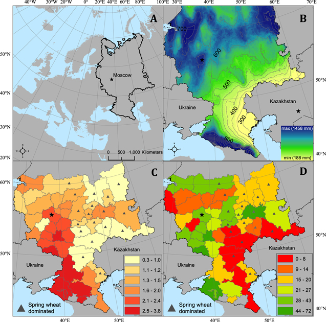
Figure 1. Study region (A); average annual precipitation (mm) (B); average wheat yields (t/ha, 1991–2012) (C); average N fertilizer use (kg/ha, 1991–2012) (D). Data sources: Climatic Research Unit (CRU, TS 1.0 and 2.0, http://www.cru.uea.ac.uk/cru/data/hrg.htm) (B); ROSSTAT (2014) (C) and (D).
Download figure:
Standard image High-resolution imageHowever, stable anticyclone circulation with dry air during the summer results in recurrent and severe droughts in southern European Russia (Dronin and Kirilenko 2008). During the 20th century, major droughts occurred in southern European Russia at least 27 times (Meshcherskaya and Blazhevich 1997). Thus, on average, every fourth year was affected by limited precipitation, which results in frequent yield declines and production shortfalls in the southern breadbaskets. Widespread irrigation networks for mitigating the impacts of drought on yields were built during the Soviet era. However, these networks have fallen into disrepair since the collapse of the Soviet Union (USDA 2013). Continental, dry weather conditions characterize the southeastern portions of European Russia (figure 1(B)) where spring wheat dominates the cropping patterns. In southeastern portions of European Russia, irrigation practices are rare and N application rates are generally low, particularly near the Kazakhstan boarder (figure 1(D)).
Since the collapse of the Soviet Union, Russia has transitioned from being a net importer of wheat (17.59 million tons (Mt) in 1992) to one of the top five net exporting countries of wheat (16.82 Mt in 2009, FAO 2013), mainly because the collapse of the Russian livestock sector reduced the domestic demand for fodder crops (Lioubimtseva and Henebry 2012, ROSSTAT 2014). However, the volatile climate conditions have caused large annual fluctuations in wheat yields, as observed in 2010 when Russia only exported 11.85 Mt of wheat (FAO 2013). The global importance of Russian wheat production is mainly attributed to its large area of wheat cultivation. Although the total cropland decreased by 35% or 41.1 Mha from 1990 to 2011 (from 117.7 to 76.6 Mha), mainly because of the contraction of fodder production, the wheat cultivation area remained fairly stable during this period (from 24.2 Mha to 25.5 Mha, ROSSTAT 2014). The average area harvested for wheat was 24.8 Mha between 2008 and 2011, which was second only to India (28.3 Mha, FAO 2013).
Between 2008 and 2011, the average wheat yield in Russia was only 2.2 t ha−1. In contrast, Germany and France achieved 7.6 and 7.0 t ha−1, respectively, during this period (FAO 2013). The average winter wheat yields in Russia decreased from 1.93 t ha−1 between 1990 and 1992 to 1.49 t ha−1 between 1994 and 1996 after the collapse of the Soviet Union, which corresponded to a decrease of 23%. In the early 1990s, the decline in winter wheat yields was driven by the collapse of state support for agriculture and the liberalization of markets, which greatly reduced the ratio of the agricultural output prices to input prices and resulted in decreased input intensity (Rozelle and Swinnen 2004). Particularly, N fertilizer use declined from 88 kg ha−1 in 1990 to 17 kg ha−1 in 1995, which corresponded to a decrease of more than 80% (figure 2). The 23% decrease in wheat yields during the early 1990s was substantially lower than the 80% decrease in N fertilizer application because the fields were often over-fertilized at the end of the Soviet era, which resulted in diminishing N returns (Liefert et al 2003). Moreover, the long-term effect from high fertilization during socialist times likely resulted in the diminished yield declines in the early 1990s (Gutser et al 2005). The increasing wheat yields after 1998 partially resulted from better weather conditions, but also resulted from the recovery of the agricultural sector and the concurrent increase of the agricultural input intensity, particularly for N fertilizer (figure 2) and high-quality seeds (Liefert et al 2010).

Figure 2. Wheat yields and nitrogen fertilizer use in Russia. Data source: ROSSTAT (2014).
Download figure:
Standard image High-resolution image2.2. Crop growth model
We applied the SWAT model to simulate potential yields. The SWAT model is a process-based, spatially distributed model that operates on a daily time step (Arnold et al 1998). SWAT has been used in various applications for quantifying the impacts of land management and climate on plant growth, yield, and hydrological parameters (Gassman et al 2007). Spatial parameterization of the SWAT model was performed by delineating a watershed into sub-basins according to topography and into hydrologic response units (HRUs) according to soil and land-use characteristics. SWAT uses daily climate data, such as precipitation, the minimum and maximum temperatures, and solar radiation, from weather stations to simulate the plant water uptake, transpiration, vegetation phenology, soil and canopy evaporation, and other hydrological components daily. The provision of solar energy drives the vegetation phenology and biomass production.
Plant growth was simulated using the crop growth component of the SWAT model, which is a simplified version of the erosion productivity impact calculator (EPIC, Williams 1995). The EPIC computes the leaf area development, light interception, and biomass conversion in the absence of biotic and abiotic limitations. The actual biomass growth is simulated by imposing stress during plant growth, including insufficient water supply, temperatures beyond the ideal crop-specific ranges, and N and phosphorus limitations. The amount of simulated aboveground biomass is converted to actual yield by multiplying it by a crop-specific harvest index that is inhibited by a water stress factor. The water stress is calculated as the ratio of actual to potential plant transpiration. According to heat unit theory, the EPIC assumes that all heat above a plant-specific base temperature accelerates plant growth and development until a temperature cut-off is reached (Neitsch et al 2011). The crop growth component of the SWAT model can reproduce observed wheat yields in various geographical settings (Faramarzi et al 2010, Ashraf Vaghefi et al 2014, Sun and Ren 2014). We used the SWAT Calibration and Uncertainty Program (SWAT-CUP, Abbaspour et al 2007) to calibrate, validate, and assess the uncertainties of the crop growth simulations.
2.3. Data
Global agricultural datasets, which include planting dates (Sacks et al 2010), amounts of irrigation (Portmann et al 2010), fertilizers inputs (FAO 2007), cropland extents (Ramankutty et al 2008), and yields (Monfreda et al 2008), have generally provided coarse and outdated information for Russia. Insufficient input data may inhibit the production of reliable yield potential estimates. Therefore, we obtained yearly data at the provincial level for winter and spring wheat yields between 1991 and 2006. In addition, N fertilizer inputs were obtained for 1993–2006 and the sowing areas of winter and spring wheat were obtained for 2006. These data were obtained from the official Russian agricultural inventories (ROSSTAT 2014). Because information regarding the dates of N fertilizer application was not available, we used the auto-fertilizer application function in the SWAT model. Auto-fertilization begins when N stress occurs in the plants. Data regarding the length of the growing season for wheat (from the date of planting to the date of harvesting) were obtained from the Rukhovich et al (2007), USDA (2013), and GOSSORT (2014).
To ensure that only the relevant wheat production systems were captured for the yield simulations, we selected 28 provinces with more than 25 000 ha under wheat cultivation in 2006, which corresponded to the most recent yield and input data. In 13 of these provinces, winter wheat dominated the cropping patterns in 2006. Spring wheat dominated in 15 provinces. In each province, we selected the sub-basin with the largest cropland area as the HRU for the crop growth simulations (figure 3).
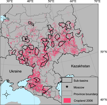
Figure 3. Selected sub-basins.
Download figure:
Standard image High-resolution imageWe extracted soil parameters from the Harmonized World Soil Database, which is a raster database with a spatial resolution of 30 arcseconds that was assembled from regional and national updates of soil information (FAO, IIASA, ISRIC, ISSCAS & JRC 2012). The climate data included monthly statistics for the total precipitation, average minimum and maximum temperatures, and the number of wet days per month (Climatic Research Unit (CRU), TS 1.0 and 2.0, http://www.cru.uea.ac.uk/cru/data/hrg.htm). Because consistent and daily data were not available from weather stations for our study area, we simulated the daily precipitation, temperature, and number of wet days per month using the monthly CRU statistics. For this simulation, a stochastic, semi-automated daily weather generator was used that generates data that well agree with the daily measured data (Schuol and Abbaspour 2007) and has been used in crop modeling (e.g., Mekonnen and Hoekstra 2011). We used the GTOPO30 digital elevation model from the US Geological Survey to delineate 546 sub-basins to obtain a realistic representation of the hydrological and agricultural characteristics for implementation in the SWAT model. The cropland patterns within each sub-basin were characterized by using data from Schierhorn et al (2013), and the dominant soil, land use, and slope options in SWAT were used to determine the hydrological parameters of each sub-basin.
Data regarding the application of other nutrient inputs (phosphorus and potassium) and pesticides were not available. However, the sensitivity analysis in SWAT suggested that the crop yields in our study region were insensitive to crop rotations and phosphorus, potassium, and pesticide inputs. Similarly, field trials in the non-Chernozem regions of European Russia demonstrated that the sensitivities of wheat yields to phosphorus and potassium applications were negligible (Kolomiec 2007). To compare the yield potentials between the provinces, we used the parameters for one spring wheat and one winter wheat cultivar from the default SWAT database and excluded wheat parameters from the calibration.
2.4. Calibration, validation, and uncertainty assessment
The SWAT-CUP was used with the integrated Sequential Uncertainty Fitting Program (SUFI-2) for the sensitivity analysis (text A1, table (A1)) and the calibration and uncertainty assessments. The SUFI-2 maps all sources of uncertainty (i.e., uncertainty related to parameters, input data, and model structure) that are related to the simulated parameters that are drawn from a sample of 500 Latin hypercube parameter values. The output range of the wheat yields that spans 95% of all simulation results represents the model uncertainty. This range is denoted as the 95% prediction uncertainty band (95PPU). The 95PPU is calculated from the cumulative frequency distribution of all of the simulated yield levels at each point in time. The lower boundary of the 95PPU represents the 2.5th percentile, while the upper boundary represents the 97.5th percentile of the distribution.
The pre-selected parameters that affected the wheat yields in each province were considered for calibration in SUFI-2 (text A2, table (A2)). To select the parameter values that resulted in the best fits between the observed and simulated yields, we began by specifying large but physically meaningful parameter ranges that ensured that the observed yield data were within the 95PPU. In subsequent iterations, the parameter ranges were narrowed to decrease the parameter uncertainty while ensuring that the observed yields remained within the 95PPU. The narrower parameter ranges were centered on the most recent and best simulation for the subsequent iterations. Iterative calibration was conducted separately for the 28 provinces to account for the large spatial heterogeneity of the geophysical and agricultural conditions in the study area (Faramarzi et al 2009). A two-year warm-up period was simulated before the validation (1991–1994) and calibration (1995–2006) periods to account for the unknown initial conditions. The warm-up period was used to equilibrate the simulated physical processes to mitigate the unknown initial conditions and exclude them from the analysis.
We used the R and P factors to quantify the goodness-of-fit of the calibration and to assess the uncertainty. The R-factor is the average thickness of the 95PPU band divided by the standard deviation of the observed yield data. The value of the R-factor ranges from zero to infinity, where zero is ideal and values of less than one are desirable. The P-factor is the percentage of the observed yield data that are bracketed by the 95PPU band (maximum value 100%). A 10% measurement error was included for all observed variables when calculating the P and R factors. We used the root mean squared error to assess the fit of the best simulation in the objective function.
2.5. Management scenarios and yield gap estimation
We used the calibrated SWAT model to simulate wheat yield potentials and wheat yield gaps using two scenarios. The first scenario (S1) assumed sufficient N fertilizer applications under rainfed conditions. The second scenario (S2) simulated conditions with sufficient N fertilizer under irrigated conditions. In this case, the yields were only influenced by the biophysical conditions and the crop cultivar. The automatic application options for N and water were used to eliminate N stress under S1, and N and water stress under S2.
We ran all simulations for every year in the calibration period (1995–2006) to capture and analyze the impacts of the annual weather conditions on the yield potentials. In both scenarios, the yield gaps for each year were calculated for 1995–2006 from the differences between the observed and simulated yield potentials of the particular year.
3. Results and discussion
On average, 78% (P-factor = 0.78) of the observed wheat yields for calibration and 82% (P = 0.82) for validation were within the simulated uncertainty bands (figures 4(A), (B), and table 1). The R-factors represented the higher uncertainty in the regions that were dominated by spring wheat (table A3). Fertilizer use was lower in most of the spring wheat regions, thus, the yields were more contingent on soil organic carbon contents and crop rotation practices in these regions (López-Bellido et al 1996). The lack of reliable soil data and crop rotation practices potentially caused the higher uncertainty that was observed in the simulated yields for the spring wheat regions.
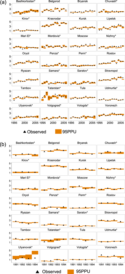
Figure 4. Comparison of observed yield (t/ha) with 95PPU of simulated wheat yield (t/ha) for calibration (A) and validation (B). Asterisk indicates areas dominated by spring wheat.
Download figure:
Standard image High-resolution imageTable 1. Calibration and validation statistics (province-level average).
| P-factor | R-factor | ||
|---|---|---|---|
| Spring wheat | Calibration | 0.82 | 1.34 |
| — | Validation | 0.82 | 1.58 |
| Winter wheat | Calibration | 0.78 | 0.64 |
| — | Validation | 0.90 | 1.06 |
Note: Calibration and validation statistics for all of the provinces are in table A3.
We obtained average (i.e., from 1995 to 2006) 95PPUs of the yield potentials for spring wheat of between 2.68 and 3.49 t ha−1 under S1 and between 4.63 and 4.82 t ha−1 under S2 in European Russia. For winter wheat, the average yield potentials were 4.30–4.63 t ha−1 under S1 and 5.45–5.58 t ha−1 under S2. The uncertainty was higher under S1 (rainfed) than under S2 (irrigated), particularly for the spring wheat regions (see also figure A1). The average winter wheat yield potentials under S2 were more than 2 t ha−1 lower than the average yield potential of winter wheat throughout Russia according to Liu et al (2007), who conducted global simulations using the EPIC model (2007). Conversely, our S2 results were approximately 2 t ha−1 greater than the estimate by Licker et al (2010), who approximated yield gaps by comparing observed and maximum yield values in locations with similar soil moisture and temperature characteristics on a global scale in 2000. However, the yield potentials based on biophysical analogs are lower. Thus, the yield gaps are smaller than those estimated from models that simulate potential crop growth under optimal conditions. Even the most advanced wheat and rice systems only approach 70–85% of the yield potential that is simulated by crop growth models. This result occurs because farmers strive to maximize profits rather than yields (Cassman et al 2003, Lobell et al 2009, Van Wart et al 2013).
The yield potentials for spring and winter wheat increased form the north to south under S1 and S2 due to the higher solar energy supply, longer growing season and better soil conditions in the south (figures 5(A), (B)). The largest and smallest yield potentials were simulated in S2 for Stavropol (6.77–6.84 t ha−1) in the south and for Vologda (4.14–4.23 t ha−1) in the north, respectively.

Figure 5. Yield potentials (t/ha) under S1 (rainfed conditions, (A)) and S2 (irrigated conditions, (B)); yield gaps (t/ha) under S1 (C) and S2 (D). All maps show averages from 1995 to 2006.
Download figure:
Standard image High-resolution imageThe average 95PPU of the yield gaps for the winter and spring wheat were 1.51–2.10 t ha−1 (44–52% of the potential yield) for S1 and 3.14–3.30 t ha−1 (62–63%) for S2. Thus, relaxing nutrient stress is important for increasing wheat yields in European Russia. For winter wheat, the average yield gaps were 1.95–2.27 t ha−1 (45–49%) for S1. The absolute yield gaps were lower for spring wheat, with 1.22–2.03 t ha−1 for S1. However, the relative yield gaps were generally higher for spring wheat (45–58%) than for winter wheat (45–49%). The yield gaps for spring wheat (3.18–3.36 t ha−1, 68–70%) were substantially greater than those for winter wheat in S2 (3.03–3.16 t ha−1, 55–57%).
The average yield gap for S2 was 65–160% greater than that of S1 for spring wheat, but only 39–55% greater for winter wheat. This difference reflected the continental climate in the spring wheat regions with lower precipitation and more frequent and intense droughts. Precipitation and the number of days per year when water stress limits plant growth (see section 2.2) affect the spring wheat yields, especially in southeastern European Russia such as in Volgograd (figure 6; the correlation between precipitation and simulated water stress days with R2 = −0.48, and between the observed wheat yields and simulated water stress days with R2 = 0.7). Water stress crucially limits potential yields under S1, particularly in the spring wheat regions. Therefore, irrigation could substantially increase the average yield potential (figure 5(B)), as demonstrated by the field experiments that were conducted in Volgograd (Grigorov et al 2007).
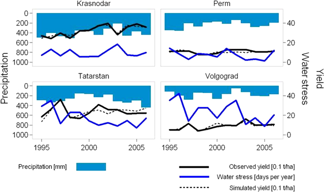
Figure 6. Annual precipitation (mm) for the growing period; wheat yields (0.1 t ha−1) and the number of days per year when water stress limits plant growth. Simulated yields and days with water stress were obtained from the best SWAT simulation.
Download figure:
Standard image High-resolution imageAt the provincial level, the average yield gaps were greater than 1.5 t ha−1 in most provinces for both S1 and S2 (figures 5(C) and (D)). For S1, the yield gaps were generally larger in northern European Russia, where the crop growth was mainly constrained by nutrient availability. Shortages in nutrient supplies and water and high daily temperature peaks limit the wheat yields in southern European Russia. We observed that the smallest yield gaps occurred in Krasnodar and Tatarstan for S1, which have fertile soils, above-average and stable precipitation (figure 6), and had above-average N applications between 1995 and 2006 (70 kg ha−1 in Tatarstan and 51 kg ha−1 in Krasnodar compared with 20 kg ha−1 for European Russia as a whole; ROSSTAT 2014).
Considerable annual fluctuations in yield potentials and yield gaps occurred for S1 (figure 7) due to the high interannual climatic volatility, particularly in the spring wheat regions in the southeastern region of European Russia (Penza, Samara, Saratov, Ulyanovsk, and Volgograd; figure 6). The high interannual volatility in the yield potential was much lower under irrigated conditions (S2, figure 7). The high volatility of potential yields under rainfed conditions underscores the importance of investigating the year-to-year variations in the regions where climate fluctuations are important for harvest outcomes. The static representations of crop yield potentials in these environments obscure the climate-driven volatility of the crop yields.

Figure 7. Observed yield and yield potentials (t/ha) under S1 (rainfed conditions) and S2 (irrigated conditions). Asterisk indicates areas dominated by spring wheat.
Download figure:
Standard image High-resolution image
The yield potentials were more stable for S1 between 1995 and 2006 in northern European Russia (e.g., Kirov, Perm, Udmurtia, Vologda; figure 7) because the precipitation patterns were less volatile and the yield reductions due to water stress were weaker. For example, the correlation between precipitation and water stress days was small in Perm (Pearson R2 = 0.19) and non-existent between the yields and the number of water stressed days (Pearson R2 = 0.01) (figure 6). However, the sowing area in the northern region of European Russia and its importance for agricultural production are relatively small. Expected climate change will most likely prolong the growing season in northern latitudes (Olesen and Bindi 2002, Kiselev et al 2013), which will result in higher future yield potentials (Dronin and Kirilenko 2011) and provide incentives for reusing abandoned agricultural lands (Schierhorn et al 2012). Increasing yield potentials and decreasing crop shortfalls due to drought suggest that northern European Russia may become a more important grain-producing region.
We detected the highest average yield gaps of up to 4 t ha−1 for S2 in southeastern European Russia along the border of Kazakhstan (Volgograd, Saratov, Penza, Samara, and Ulyanovsk; figure 5(D)). The yield potentials and yield gaps in this region were substantially lower under S1 (rainfed) than under S2 (irrigated) in most years (figure 7). In this case, increasing N application will not increase the yield potentials due to the crop-water limitations, which are similar to the co-interactions between yields, fertilizer, and water availability in the Australian breadbasket (Bryan et al 2014) and rainfed Mediterranean regions (López-Bellido et al 1996). Moreover, the high annual volatility of precipitation (figure 6) and the ensuing frequent crop failures contribute to the observed low applications of intermediate inputs (fertilizer, in particular) because the agriculture profits become highly uncertain in the absence of adequate agricultural insurance schemes (Dronin and Kirilenko 2011, Kiselev et al 2013). One promising avenue for increasing and stabilizing yields in the regions with high climatic volatility is the development and cultivation of drought-resistant wheat varieties (Howden et al 2007, Grabovets and Fomenko 2008, Challinor et al 2014). Improved crop rotations and no-till practices are relevant adaption strategies for climate change (Smith and Olesen 2010, Aguilera et al 2013).
Unfortunately, no data are available at the pan-Russian scale that allows us to include crop varieties and crop rotations in the simulations. Therefore, we disregarded alternative crop rotations and we relied on the simplified representation of wheat varieties with the default wheat parameters of the SWAT model, akin to other large-scale crop simulations (Bondeau et al 2007, Liu et al 2007, Nelson et al 2010). This prohibited us from analyzing the effect of different wheat varieties and rotations on wheat yields, but it permits between-site comparison of yield potentials subject to the climate signal and to regional management.
4. Conclusions
Crop yields were low and the yield gaps were high across most of the fertile agricultural lands of European Russia. Unfortunately, little conclusive evidence has been obtained regarding the potentially attainable yields and the drivers of the yield gaps in European Russia. To address this gap, we simulated the annual wheat yield potentials for European Russia between 1995 and 2006 using a crop growth model that was calibrated with provincial-level agricultural inventory data. On average, yield gaps were 1.51–2.10 t ha−1 and 3.14–3.30 t ha−1 for rainfed and irrigated conditions, respectively. The yield gaps varied considerably across space and time, driven by the high interannual volatility of the precipitation patterns and the input intensity.
Despite the large yield gaps, we caution against exaggerated yield expectations. First, yield potentials decrease substantially during drought years, particularly in the breadbaskets of southern Russia where the climatic conditions are volatile and the current cropping systems are mainly rainfed. The yield gaps under irrigated conditions are highly speculative and depend on the available water resources and on the economic feasibility of expanding the irrigation capacity. The high likelihood of drought has important implications for farm entrepreneurs who aim to maximize their profits rather than yields because investments in intermediate inputs, such as fertilizer, are lost during drought years when the yields collapse.
Policies that improve agricultural insurance schemes may successfully reduce the investment risks in the Russian breadbaskets, which would increase input intensity and production. In addition, strategies that incentivize the use of existing water resources and improve the efficiency of water use may enhance production. Such initiatives will become increasingly important as the frequency of summer drought and heat stress increase with future climate change (Alcamo et al 2007, Kiselev et al 2013), which would lead to higher crop yield volatility. Our results are helpful for quantifying potential crop production and for pinpointing management strategies and research initiatives that will help improve yields and close yield gaps in this globally important agricultural region.
Acknowledgments
This manuscript has benefited from the contributions of A Balmann, J K Thakur, S Neumann, M Volk, F Witting, and M Strauch. We are grateful for the financial support of the Leibniz Association's 'Pakt für Forschung', the German Federal Ministry of Education and Research (BMBF) (Code01 LL0901A), the German Federal Ministry of Food and Agriculture (BMEL) (GERUKA), and the European Union (FP7-ENV-2010-265104).