
Abstract
This study compares seasonal and spatial variations in methane fluxes as sources of uncertainty in regional CH4 flux upscaling from the wetlands of West Siberia. The study examined variability in summertime CH4 emissions from boreal peatlands, with a focus on two subtaiga fen sites in the southern part of West Siberia (Novosibirskaya oblast). We measured CH4 flux, water table depth, air and peat temperature, pH and electric conductivity of peat water during three field campaigns in summer 2011 (9–12 July, 26–28 July and 20–21 August). Fluxes were measured with static chambers at sites chosen to represent two of the most widespread types of wetlands for this climatic zone: soligenous poor fens and topogenous fens. In both sites the water table level acts as the primary control on fluxes. For the poor fen site with good drainage, water table controls CH4 fluxes on the seasonal scale but not on a local spatial scale; for the fen site with weak drainage and microtopographic relief, the water table controls fluxes on the local spatial scale, but does not drive seasonal variations in the flux magnitude. This difference in hydrology shows the necessity of including detailed wetland type classification schemes into large-scale modeling efforts. From these three measurement periods, we estimated the relative seasonal variation in CH4 emissions as 8% for the fen site and 26% for the poor fen site. These results were compared to estimates of other sources of uncertainty (such as interannual variation and spatial heterogeneity) to show that quantifying seasonal variability is less critical than these other variations for an improved estimate of regional CH4 fluxes. This research demonstrates and ranks the challenges in upscaling measured wetland CH4 fluxes across West Siberia and can guide future field campaigns.
Export citation and abstract BibTeX RIS

Content from this work may be used under the terms of the Creative Commons Attribution 3.0 licence. Any further distribution of this work must maintain attribution to the author(s) and the title of the work, journal citation and DOI.
1. Introduction
High-quality, quantitative estimates of the CH4 budget are crucial to predicting climate change, managing Earth's carbon reservoirs, and understanding atmospheric chemistry (Mikaloff-Fletcher et al 2004). Therefore, the contribution of different sources to the atmospheric concentration of CH4 is important to determine in addressing the problem of global warming (Heimann 2011). Since wetlands are considered to be the major natural source of methane, accurate estimation of their emissions at the regional scale is required (Fung et al 1991) though a recent model inter-comparison project still reveals significant disagreement in simulated CH4 emissions (Melton et al 2013).
West Siberia has a special importance in this respect as it is one of the most paludified regions in the world with a mire area of 68.5 Mha or 27% of the region's area (Peregon et al 2009). However, several estimates based on field studies exhibit a large spread in annual regional fluxes, from 2 (Bleuten 2007) to >22 MtCH4 yr−1 (Panikov 1995), as reviewed previously (Glagolev et al 2012). Closer examination of these studies (Glagolev et al 2008) attributed this uncertainty to a lack of field measurements. Furthermore, the extrapolation of higher flux measurements taken in southern zones to northern zones has likely generated over-estimates at the higher end of the range (Bohn et al 2013). Aiming at the reliable estimation of the regional emission from West Siberia mire systems, a long-term (2007–2011) and large-scale (from forest steppe to tundra wetlands of Western Siberia) investigation was organized resulting in a narrower estimate range of 2.6–5.2 MtCH4 yr−1 (Glagolev et al 2011). This estimate was obtained using an inventory concept of methane emissions (Glagolev et al 2011), and using the so-called standard model (Glagolev et al 2012). This model generates a bottom-up estimate of West Siberian wetland methane emissions by multiplying the average emission rates of each mire ecosystem type with the area coverage of these ecosystems and accounts for changes in the length of the peak methane production period for each zone.
Such bottom-up inventories are susceptible to several categories of errors leading to the incorrect evaluation of the resulting flux estimate:
- unrepresentative data about methane fluxes caused by a limited number of potentially non-representative field observations and strong flux variability among the different sites and observation periods;
- the low quality of wetland maps upon which to define the relative area of different wetland ecosystems;
- uncertain estimates of the length of the methane emission period (MEP).
In this study we do not take into consideration errors introduced by potential mistakes in mapping (Frey and Smith 2007) and rely on a map of West Siberia dividing the region into 8 bioclimatic zones and reducing of the natural range of wetland forms to 8 wetland typologies (Peregon et al 2008, 2009). Of the contributors to upscaling uncertainty, we analyze questions of flux variability and the duration of the MEP. We compare uncertainties in the regional flux estimate from the following four contributing factors:
- interannual variability;
- seasonal variability (caused by seasonal changes of the environmental factors controlling CH4 emissions);
- variability among different mires (caused by local climate, hydrology or geochemistry);
- spatial variability within the mire ecosystem (caused by local microrelief, plant or microbial communities).
In this study attention is paid to contributors of both spatial and seasonal variability. There are only a few studies of the seasonal variability of methane emission from Russian mires. Most of these studies have focused on tundra mires (Nakano et al 2000, Heikkinen et al 2002, 2004, Wagner et al 2003, Sachs et al 2010, etc) and the south taiga zone of Western Siberia (Friborg et al 2003, Krasnov et al 2013). In other climate zones the seasonal dynamics have not been studied specifically despite comparatively high methane emissions and seasonal changes in water temperature and phenology, including middle and north taiga wetland lakes (Repo et al 2007), forest–tundra and north taiga bogs (Naumov et al 2007), and forest-steppe bogs (Naumov 2011). The relative weight of the climate factors driving seasonal variations in methane emissions may also differ between zones. For example, the period when emissions from wet sites exceed 2 mgCH4 m−2 h−1 has been estimated as 70 days for a tundra site (Heikkinen et al 2004) and 125 days for a south taiga site (Friborg et al 2003) even though the mean July fluxes are similar for these sites (about 7.5 mgCH4 m−2 h−1). In this sense, extrapolation of seasonal dynamics obtained in one zone to another zone could lead to a critical bias in the regional estimate. Thus, it is necessary to investigate seasonal dynamics in each climatic zone, an investigation missing in previous work (including Glagolev et al 2011). In this paper we estimate uncertainty deriving from seasonal variations in methane emissions and try to understand how knowledge of these variations improves the regional CH4 flux estimate from West Siberian wetlands in comparison with other sources of uncertainty. Then several weak points of the inventory method are examined by comparing different contributors of uncertainty and suggest an optimal field campaign strategy.
The objectives of the study were (i) to quantify the uncertainty in the flux estimation caused by the seasonal variation of environmental parameters in a case study from two study sites within the subtaiga zone (a zone of deciduous birch-aspen forests); (ii) to compare the relative importance of different contributors to uncertainty on the regional flux estimate and (iii) to identify the main controlling factors which influence seasonal dynamics of CH4 fluxes.
2. Materials and methods
2.1. Test sites
The field experiments were carried out during the 2011 summer period. For comparability, these measurements were taken in the same season as the majority of the measurements in a previous study (Glagolev et al 2011): 9–12 July, 26–28 July and 20–21 August. Methane fluxes were measured at two test sites in the subtaiga zone of Western Siberia: 'Biaza' (56.50°N, 78.31°E) a topogenous fen, and 'Chuvashi' (56.41°N, 78.80°E), a soligenous poor fen, according to a Russian mire classification scheme (Masing et al 2010). Detailed test site descriptions are in appendix
2.2. Study methods
2.2.1. CH4 flux measurements
CH4 exchange to the atmosphere was measured using the static, opaque chamber method, in 82 measurements each at the fen and poor fen mires. Of these measurements, triplicate measures at each chamber site were taken to average short-term variations in flux strength. The chamber consisted of two parts: (i) a permanent stainless steel square collar (40 cm × 40 cm, embedded 15 cm into the peat surface), and (ii) a removable plexiglass box (30 or 40 cm height). To minimize the changes of chamber temperature, the plexiglass box was covered with reflecting aluminum fabric. Mechanical disturbances of the peat layer were minimized by using portable or permanent footbridges.
The fan-mixed chamber headspace was sampled at four equal intervals and the CH4 concentration in these samples was measured on a calibrated gas chromatograph (see appendix
At each site the following environmental characteristics were measured: air and peat temperatures (at the depths of 0, 5, 15, 45 cm) by the temperature loggers 'TERMOCHRON' iButton DS 1921–1922 (DALLAS Semiconductor, USA), pH and electrical conductivity by a Combo 'Hanna 98129' ('Hanna Instruments', USA) and concentration of dissolved oxygen by an 'Ecotest-2000' ('ECONYX', Russia). Botanical descriptions were also made to describe the vegetation community within each chamber site.
2.2.2. Data analysis
The STATISTICA 8 software ('StatSoft', USA) was used for statistical analyses. Ordinary-least square regression (α = 0.05) is used to determine the significance of the relationship between the environmental variables and measured CH4 flux (averaged across the three temporal replicates). Stepwise multiple regressions (α = 0.05) included parameters for air Tair and peat temperatures T0, T5, T15, T45 at the depths of 0, 5, 15, 45 cm respectively (°C), minimal, mean and maximal pH and electric conductivity (μS cm−1) pHmin, pHmean, pHmax, ECmin, ECmean, ECmax, and water table level WTL (cm). The variables from this list that were not statistically significant were omitted from the reported results of the multiple regression analyses.
2.2.3. Mire ecosystem concept
The objectives of this study are based on an assumption that even in complex mire landscapes, areas that are similar in geochemical and hydrological conditions and have homogeneous vegetation cover can be distinguished. Consequently, these areas have similar methane production and consumption rates. In this study these units are called 'mire ecosystems'. This term is equivalent to the term 'mire micro-landscape' used in Peregon et al (2008, 2009) and Glagolev et al (2011). From the diversity of mire ecosystems, in this study we focused only on fens (various types of minerotrophic fens, poor fens and wooded swamps). The full diversity of Russian mire ecosystems has been described elsewhere (Masing et al 2010).
2.2.4. The methane emission period model
The inventory concept (as well as other inventories, for example, Bartlett and Harriss 1993, Christensen et al 1995, Wang et al 2005) accounts for seasonal variations of methane emissions by dividing the year into three periods (Suvorov and Glagolev 2007). The methane flux is first assumed to increase from winter to summer and then after peaking it regularly decreases (figure 1). In the modeled version a step function is used to represent this seasonality, where the flux is
- (a)zero: from the beginning of the year to the day τ corresponding to the beginning of the methane emission period (MEP);
- (b)the flux median for each mire ecosystem types in each climatic zone: from τ to τ + MEP, corresponding to the end of MEP;
- (c)zero: from τ + MEP to the end of the year.

Figure 1. Schematic representation of the step function approach for approximation of seasonal CH4 flux dynamics (see text for details).
Download figure:
Standard image High-resolution imageThe parameters defining the MEP were chosen on (1) the basis of the biologically active period whose start is determined from the date when mean daily air temperature becomes higher than 10 °C and ends the when mean daily temperature becomes lower than 0 °C (Rihter 1963) and (2) the analysis of seasonal variations in methane flux from several south taiga wetlands. For the south taiga zone, the MEP was calculated as the ratio of the total emission in the snow-free period (calculated by a numerical integration of the methane emission curve during the snow-free period) and the median flux from the same wetland and was about 10% longer than the biologically active period (Suvorov and Glagolev 2007). Because the MEP is derived from the median value of the flux measurements and the integrated annual flux, asymmetry in the flux measurement distribution would not distort the use of the median (Glagolev et al 2010). The MEP values for other zones were calculated assuming that their MEP value is proportionately larger than the biological activity period by as much as the MEP value is larger than biological activity period in the south taiga.
3. Results
3.1. CH4 fluxes
Fluxes from the two field sites are reported in appendix
Table 1. Dynamics of CH4 fluxes and their main environmental controls (± standard deviation) during the 2011 summer period (negative or positive values of the water table level (WTL) correspond to situations when WTL is lower or higher than the mean level of the moss surface, respectively).
| 9–12 July | 26–28 July | 20–21 August | ||||
|---|---|---|---|---|---|---|
| Parameter | Fen | Poor fen | Fen | Poor fen | Fen | Poor fen |
| Median of CH4 flux (mgCH4 m−2 h−1) | 2.89 ± 0.39 | 0.89 ± 0.29 | 3.24 ± 0.98 | 1.62 ± 0.68 | 3.56 ± 0.49 | 1.31 ± 0.34 |
| Number of measurements | 28 | 36 | 36 | 27 | 18 | 19 |
| Mean WTL (cm) | −0.3 ± 1.3 | −16.5 ± 2.9 | 3.7 ± 3.9 | −11.4 ± 2.9 | 5.6 ± 1.4 | −13.7 ± 4.1 |
| Mean temperature at 5 cm depth (°C) | 14.0 ± 0.1 | 15.4 ± 0.3 | 15.2 ± 1.5 | 15.7 ± 0.8 | 12.2 ± 0.2 | 16.5 ± 1.6 |
| Mean temperature at 15 cm depth (°C) | 13.1 ± 0.2 | 12.3 ± 0.2 | 13.3 ± 1.1 | 14.1 ± 0.9 | 11.0 ± 0.1 | 13.2 ± 0.2 |
| Mean pH of peat water for upper 50 cm of peat | 6.36 ± 0.10 | 4.78 ± 0.18 | 6.26 ± 0.12 | 5.15 ± 0.09 | 6.1 ± 0.15 | 5.38 ± 0.11 |
| Mean EC of peat water for upper 50 cm of peat (μS cm−1) | 133 ± 19 | 43 ± 19 | 121 ± 24 | 48 ± 20 | 149 ± 33 | 42 ± 10 |
Typically, the uncertainty of the individual measurements was around ±0.2 mgCH4 m−2 h−1 for both sites, with the highest uncertainty contributed by scatter in the measured gas concentrations. The temporal variability within the test site was estimated as the standard deviation of the average across the three measurements taken in a row (i.e., within 1.5 h) and was also around 0.2 mgCH4 m−2 h−1.
3.2. Seasonal variability
The relative seasonal variability (calculated as the ratio between the standard deviation of the median flux of each measurement session to median fluxes across the whole season) were 26% and 8% for the poor fen and fen, respectively. The significantly higher seasonal flux variations in the poor fen derive from seasonal fluctuations of the water table level. In the second half of July precipitation in this region was high (about 120 mm) and resulted in a ∼40 mm rise in the water table of both study sites (see table 1). At the end of August the hydrological conditions were changed: the poor fen with the better drainage became slightly dryer, while the inundation level of the weakly drained fen continued to grow. Thus, the water table level of the poor fen varied more widely across the measurement period. Since both mires have similar regression lines between CH4 flux and water table level, their hydrological differences resulted in a higher variability of methane emissions in the poor fen.
3.3. Controls on CH4 fluxes
Regression analysis revealed that it was possible to construct a multidimensional model with independent and significant parameters for all microsites as well as separately for the fen and poor fen (figure 2). The model for all microsites (Fa, mgCH4 m−2 h−1) contains WTL and T15:
The model of CH4 fluxes in the fen (Ff, mgCH4 m−2 h−1) also contains WTL and T15 as explanatory variables:
For the poor fen (Fpf, mgCH4 m−2 h−1), WTL and pHmean are the key explanatory variables:
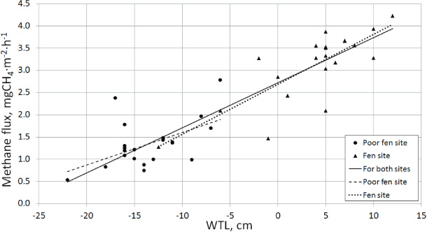
Figure 2. Individual water table level versus CH4 flux (the median flux of each triplicate measurement session at each chamber site). All relationships are significant (α = 0.05). Regression lines are shown for both sites ((CH4 flux) = (0.10 ± 0.01)(WTL) + 2.72 ± 0.08, R2 = 0.82), for the poor fen site ((CH4 flux) = (0.07 ± 0.03)(WTL) + 2.33 ± 0.38, R2 = 0.28), for the fen site ((CH4 flux) = (0.11 ± 0.02)(WTL) + 2.68 ± 0.13, R2 = 0.64).
Download figure:
Standard image High-resolution imageA simple one-dimensional regression reveals that for both sites as well as for each site separately WTL is the single best predictor of emissions (where the median flux for the three temporal replicate measurements is used; see table 2). For the poor fen site, the peat water chemical characteristics (EC and pH) are also significant. Conversely, for the fen site only T5 and T15 are also significant. The highest deviations from the WTL regression curve for the fen site (i.e., the two significantly lower values) may be caused by the relatively small coverage of vascular plants (10–20%) compared to the other points whose coverage is more than 30%. For the poor fen site, the substantially higher and lower residuals were correlated with the highest and the lowest values of pHmax, respectively.
Table 2. Coefficients of determination of simple regressions between environmental parameters and CH4 flux for the sites grouped together and for each site separately. Bold font indicates the significance level (α = 0.05).
| Environmental variable | Both sites | Poor fen | Fen |
|---|---|---|---|
| WTL | 0.82 | 0.28 | 0.64 |
| Tair | 0.27 | 0.07 | 0.04 |
| T0 | 0.39 | 0.01 | 0.15 |
| T5 | 0.31 | 0.01 | 0.21 |
| T15 | 0.15 | 0.01 | 0.25 |
| T45 | 0.54 | 0.16 | 0.21 |
| pHmin | 0.55 | 0.23 | 0.12 |
| pHmean | 0.46 | 0.26 | 0.19 |
| pHmax | 0.58 | 0.27 | 0.12 |
| ECmin | 0.35 | 0.19 | 0.19 |
| ECmean | 0.49 | 0.22 | 0.11 |
| ECmax | 0.44 | 0.14 | 0.15 |
4. Discussion
4.1. Seasonal variability
The seasonal variation of our methane flux data is 8% for the fen with weak drainage and 26% for the poor fen site with relatively good drainage. Similar calculations using various published data (Heikkinen et al 2002, 2004, Friborg et al 2003, Ding and Cai 2007) give the seasonal variation of 11–30% (see table 3). For the fen intermediate flark site (Heikkinen et al 2004) the relative seasonal variability is 11% and for non-degraded and slightly degraded polygon tundra sites (Sachs et al 2010) it was 21% and 16%, respectively. Because other fen sites even in different climatic zones also have seasonal variability sufficiently less than 30%, this low variation may be presumed to be a general pattern for fens. In their general characteristics these mires are similar—they all are fens on watersheds with relatively shallow peat depth and weak drainage (caused by clay parent rock or permafrost). In general the bell-shaped curve of methane emission for Western Siberia mires has two main contributors, which are the similarly shaped seasonal precipitation and air temperature curves (Heikkinen et al 2004, Naumov et al 2007, Naumov 2011). Such a pattern is typical for all regions with a continental climate.
Table 3. Comparison of different sources of CH4 flux variability for West Siberian and ecologically similar wetlands.
| Type of variability | Level of relative variability |
Contributing flux range |
Number of contributing measurements | References | Notes |
|---|---|---|---|---|---|
| Interannual variability | ±61 | 2–6 | 200 | Heikkinen et al (2002, 2004) | For 2 years (season average fluxes) |
| ±40 | 3–15 | — |
Sasakawa et al (2012) | For 5 years (season average fluxes) | |
| ±26 | 5.7–19.4 | 220 | Panikov and Dedysh (2000) and Friborg et al (2003) | For 6 years (July average fluxes) | |
| Intraseasonal variability |
±8 | 0.5–2.8 | 82 | This study | Fen site |
| ± 26 | 1.2–4.3 | 82 | Poor fen site | ||
| ±11 and ±28 | 1–12 | 46 and 46 | Heikkinen et al (2004) | For 2 mires | |
| ±21 and ±16 | 0.2–11.5 | 111 and 114 | Sachs et al (2010) | For 2 sites | |
| ± 29 | 1–11 | 80 | Friborg et al (2003) | ||
| ± 30 | 1–50 | 82 | Ding and Cai (2007) | ||
| Variability among different mires | Remains uncertain, may be more then | 0.05–4.0 | 48 | Glagolev et al (2010) | For 4 mires |
| 0.04–9.7 | 53 | Glagolev et al (2012) | For 2 mires | ||
| Spatial within mire ecosystem | ± 50% | ||||
| ±(20–30) | 0.3–10.7 | 81 | Glagolev et al (2012) | For 26 sites in 4 mires | |
| ± 35 | 1.2–7.6 | 240 | Sabrekov et al (2011) | For 9 sites in 1 mire |
aThe level of relative variability is defined as one half of interquartile range divided by median of methane flux sample and multiplied by 100% (a nonparametric analog of coefficient of variation) and the size of sample is presented in column 'Notes'. bThe contributing flux range is the range of flux values in each portion of the dataset used to derive the level of relative variability. cNot available because in this work the methane emissions measured in 2005–2009 at two different sites were calculated using inverse modeling. dIntraseasonal variability was calculated for the period for which the majority of flux data used for inventory in Glagolev et al (2011) was obtained—for late June–late August period.
At this study's poor fen site, where water continuously drains from the mire during the summer period, the methane emissions generally follow the changes in WTL. This relationship has also been discovered for the poor fen site in Friborg et al (2003) and the bog site in Ding and Cai (2007). As an example, the seasonal dynamics from Friborg et al (2003) were successfully predicted with a WTL model (Bohn et al 2007). But if the drainage from a fen is very poor, then there is often no significant correlation between WTL and CH4 flux and only temperature acts as a control of emission (e.g., Heikkinen et al 2004, Sachs et al 2010). Thus based on the available data two types of seasonal emission dynamics could be defined:
- (1)
- (2)
The sites in our study also are in agreement with this pattern (see below in section 4.4). It additionally should be noted that local weather conditions and climatic anomalies can change this general pattern. However, the two divergent seasonal flux–WTL patterns should encourage the inclusion of detailed wetland type classification schemes into large-scale modeling efforts because different wetland types can have opposite responses to changing climate characteristics.
4.2. Comparison with other sources of variability
An estimate of seasonal variability can be compared with other sources of variability to determine the greatest contributor to uncertainty in the regional flux estimate. This comparison can help to generate more effective field campaigns to improve the quality of regional flux estimates. Contributions of other types of variability were determined using measurement data from a methane emissions database (Glagolev et al 2011) and elsewhere and are synthesized in table 3. The potential influence of diurnal variability was not analyzed in contrast with studies from China (Ding and Cai 2007), because significant evidence of CH4 flux diurnal variations have not been found in previous West Siberian studies (Heyer et al 2002, Sabrekov et al 2011).
Unfortunately, there are not enough data to estimate variability among different mires properly. This type of variability is especially hard to determine in the field because fluxes in different places should be measured at more or less the same time. With the unknown strength of inter-mire variability and the high contribution of local heterogeneity in flux upscaling (table 3), we conclude that for regional flux estimates the spatial coverage of a field investigation is more critical than temporal coverage. We can then advise as a best strategy that field campaigns should investigate more sites with only a few days of observations per site. There may be diminishing benefits to conducting more than 50–70 flux measurements on each site, since according to table 3 this number is adequate to represent spatial variability within mire ecosystems and a greater number of measurements is not necessary. Improvements in constraining site-to-site variations in flux strength should lead to improvements of the regional flux estimate because they allow the aggregated flux estimate to incorporate spatial variations within the ecological diversity of mires. It will help to remove the highest uncertainties in the regional flux estimate despite the continued difficulty in accounting for interannual (including climate-related trends) and interseasonal variations.
The fact that spatial variability is of more importance than temporal variability implies that such factors as local hydrology, geochemistry, and plant community are more important than seasonal variations in environmental conditions. These factors can vary among different mires within one climatic zone (Glagolev et al 2010, 2012) and also within a single mire (Wagner et al 2003, Kutzbach et al 2004, Kao-Kniffin et al 2010), and hence should be evaluated with a spatially oriented sampling approach. These local factors may also be particularly susceptible to climate changes that induce shifts in vegetation community and regional hydrology. Furthermore, an emphasis on greater spatial, rather than temporal, coverage during field investigations may allow the detection of methane emission hot spots that can have proportionately large impacts on the regional estimate. This approach may generate a trade-off with 'hot moments' of flux emissions, such as through ebullition, although these events are often also missed in temporally intensive campaigns (Stamp et al 2013).
4.3. Other questions of seasonal dynamic variability
The seasonal variability of methane emissions needs analysis from some other points of view, including whether the step function approach is justified for climatic zones outside the south taiga. In this respect a comparison between the most northern (tundra) and the most southern zone (forest steppe) of West Siberia can be instructive. For the tundra zone the comparison can be based on measurements carried out near Vorkuta in the European part of Russia near the border with West Siberia (67.38°N, 63.37°E) (Heikkinen et al 2002, 2004). These studies indicate MEP values (95 days) similar to the MEP of 101 days used in Glagolev et al (2011). Wetlands of north-eastern China (47.58°N, 133.52°E) are close to the forest-steppe mires of Western Siberia by their climatic conditions (see the methane flux measurements in Ding and Cai 2007). For these mires the calculated value of MEP ranges between 195–210 days; thus slightly higher than the MEP of 196 days taken for forest steppe in Glagolev et al (2011). Therefore we can conclude that the MEP values reported in our previous regional flux estimate are reliable and therefore median is here a more statistically robust characteristic than the mean.
Another critical question is whether the method generates an overestimation of the regional flux because the median flux is calculated for the months with the most intensive methane emissions and is further multiplied by the MEP as calculated from flux data from the full snow-free period. The majority of the measurements used to calibrate the model (Glagolev et al 2011) were carried out during the period from late June to early September. In reality, methane fluxes become higher than the mean winter flux earlier (from April to beginning of June, depending on climatic zone) and decrease again only after the measurement period (i.e., from September to November, also depending on climatic zone). To determine this excess seasonal methane flux variation, data from other studies were analyzed. On a preliminary basis, our data was linearly interpolated on a daily basis to compensate for data gaps in different parts of the emission season. Other studies have suggested that the ratio of median fluxes for the entire snow-free period to the period from the end of June until the beginning of September was 0.8 for tundra mires (Heikkinen et al 2004), 0.65 for south taiga mires (Maksyutov et al 1999) and 0.54 for the Chinese analog of Siberian forest-steppe mires (Ding and Cai 2007). The reduction of this ratio from north to south probably results from the longer period of ideal methane production in the more southern zones. Thus, the artificial overestimation caused by measurements conducted in the most intensive periods of methane emission may be 20–45%, with greater errors in more southern climate zones.
Another question, arising from lack of flux data in spring and autumn periods, is the reliability of the estimate of seasonal variations. Of course when the wider time range is considered a higher level of seasonal variation is obtained: methane emissions starts from near-zero fluxes in the spring and decrease to near-zero in autumn. It is important to mention that our work is not about seasonal dynamics of methane emissions directly but about the influence of these variations on the regional flux estimate. The changes of the total warm season flux (which is the area under the curve of season emission) are determined due to uncertainties deriving from the seasonal dynamics of methane emissions. All of the data for the previous regional flux estimate (Glagolev et al 2011) were obtained for the late-June–late-August period and so the estimate of seasonal variability should be calculated within this time. According to the MEP concept the exact variation in fluxes from spring to autumn is not important, rather it is important how fluxes vary within the period for which our flux data was obtained. Of course, this period should not be very short. The summer flux is the largest part of the warm season flux (as described above it composes 65–90% of the total flux depending on the climatic zone). Thus, a lack of flux data in the spring and autumn periods is less critical for our analysis. But, for example, if the flux and seasonal variability had been measured only in July, it would become critical for the total warm season flux and variability estimation because the July flux is not the biggest part of the warm season flux. Calculating the potential overestimation in this case would also be statistically unfounded.
Seasonal methane flux dynamics are more or less symmetric relative to the maximum of the methane emission for West Siberia mires (this study, Maksyutov et al 1999, Friborg et al 2003 and Heikkinen et al 2004) or for ecologically similar mires from other regions (Ding et al 2004, Ding and Cai 2007). Taking into account this fact and the overestimation described above we can make a conclusion about the time of year when the observation would be most accurate from the seasonal dynamic point of view if it is possible to only observe fluxes on a few days of the year per site. These 'optimal' times are the end of the June through the beginning of the July and the second half of August. Measurements taken in these periods would both exclude the overestimation described above and will account for nearly all seasonal variations in flux strength. While this approach has some uncertainty, if the level of seasonal variability is not higher than 30% then the benefits of higher spatial coverage outweigh the potential error in temporal coverage.
4.4. Controls of CH4 emissions
It was observed that CH4 fluxes increased significantly with increases in the water table. This finding is generally expected because lower water table levels favor aerobic respiration and CH4 oxidation (Dise et al 1993, Bubier et al 1995). A reduction in methane fluxes with increasing T15 does not fit a directly causal pattern (see Dise et al 1993 and Pelletier et al 2007 for counter observations) but can be caused by evapotranspiration. It has been suggested that greater evapotranspiration under the influence of higher soil temperatures will lower the water table and hence methane fluxes will decline (Moore and Roulet 1993, Ehhalt et al 2001). Also hummocks with lower WTL (and hence CH4 flux) tend to have higher peat temperatures (see appendix
The sensitivity of CH4 fluxes in subtaiga mires to WTL fluctuations (both in the multidimensional and one-dimensional models) was slightly higher than for mires of the same type in New Hampshire, USA (Treat et al 2007). Probably in the New Hampshire study the reduced fluxes result from a low WTL (30–40 cm below the surface) which results in a larger aerobic zone conducive to methane oxidation (see Kalyuzhnyi et al 2009). Fluctuations of WTL in this range do not play a significant role in the CH4 flux. For example, in a previous peatland study (Pelletier et al 2007) WTL varied in range −30 to 20 cm, as well as in our investigation, and the coefficients are similar (0.10–0.13).
Generally, in our flux measurements we have both types of variability: seasonal and spatial within the mire ecosystem. To distinguish them the simple one-dimensional regression between CH4 flux and WTL for each site for each of three sessions is provided (see table 4).
Table 4. Coefficients of determination (R2) of a simple regression between WTL and CH4 flux for each test site and three measurement sessions. Bold font denotes significance (α = 0.05).
| Period | Poor fen (R2) | Fen (R2) |
|---|---|---|
| 9–12 July | 0.27 | 0.86 |
| 26–28 July | 0.36 | 0.71 |
| 20–21 August | 0.26 | 0.49 |
A comparison between the coefficients of determination in table 4 and table 2 reveals that for the fen site on the local spatial scale the correlation between WTL and CH4 flux is as strong and significant as for whole fen site's combined data (where R2 = 0.64, see table 2). Hence for the fen site the spatial variability of WTL is more important than seasonal changes in WTL. For the poor fen the WTL-flux relationship within a single measurement period is insignificant but taken together across the season, the correlation is significant (see table 2). Therefore, for the poor fen site the significance of the WTL-CH4 relationship derives from correlated seasonal changes in both WTL and CH4 flux while spatial variations for each measurement session do not generate significant correlation between WTL and CH4 flux. However, the seasonal and spatial coefficients of determination are very similar, so both these potential sources of uncertainty should be considered.
The higher correlations between CH4 flux and environmental controls for both sites together rather than for each site separately (see table 2) may be explained by the higher importance of spatial variability in methane flux than seasonal variability—combining the datasets significantly increases the spatial sampling range while similar seasonal characteristics affect each site. The alternate explanation is that these findings are just an artifact of including only two mires that differ in mean flux and WTL values. The following normalization procedure was used to test these ideas: we compute the anomalies of CH4 flux and environmental variables relative to long-term mean values of these quantities at each site and then compute a two-wetland simple one-dimensional correlation between the flux and driver anomalies. In this approach only the correlation with WTL was significant (the coefficient of determination (R2) is 0.51). So for all variables from table 2 the higher correlations derived from combining the two peatlands are artifacts from combining two quite different mires.
5. Conclusions
The level of relative seasonal CH4 flux variability for West Siberian mires in the subtaiga zone is 8% for the study's fen site and 26% for the poor fen site. Comparisons between our field data and other studies reveal at least two patterns of seasonal CH4 flux variability typical for mires with different hydrological characteristics. Therefore the inclusion of more detailed wetland type classification schemes into large-scale modeling efforts should be encouraged. A comparison with other types of variability shows that seasonal variability is of less magnitude than interannual and spatial variability. These findings allow us to suggest that for regional flux estimates the spatial coverage of a field investigation is more important than temporal coverage. Thus we advise as a best field campaign strategy to investigate more sites (with only a few days of observations per site) and make not more than 50–70 well-chosen flux measurements on each site. While interannual and intraseasonal variability may also have some importance, improvements in the regional flux estimate from increased spatial coverage may produce similar reductions in the uncertainty window with less time and resources than a time-intensive multi-annual or multi-seasonal campaign.
Acknowledgments
Research has been carried out within the grant in accordance with Resolution of the Government of the Russian Federation no 220 dated April 09, 2010, under agreement no 14.B25.31.0001 with Ministry of Education and Science of the Russian Federation dated June 24, 2013 (BIO-GEO-CLIM).
B R K Runkle is supported through the Cluster of Excellence 'CliSAP' (EXC177), University of Hamburg, funded by the German Research Foundation (DFG). B Runkle thanks EU COST Action ES0902 'PERGAMON' for travel support and receives additional fellowship support from the University of Hamburg's Center for a Sustainable University. S Maksyutov is supported by the Environment Research and Technology Development Fund (2A-1202) of the Ministry of the Environment, Japan. We thank three anonymous reviewers whose ideas significantly improved the paper.
Appendix A.: Detailed test site description
- (1)'Biaza' (56.50°N, 78.31°E) is located 10 km south from the Biaza settlement between the Tartas and Tara Rivers on a weakly drained watershed. This territory is occupied by fens dominated by tussock-forming sedges (Carex cespitosa, Carex acuta) and mosses (see figure A.1); the depth of the peat layer is less than 40 cm. Mire plants are mainly dependent on atmospheric nutrient supply, but because of the shallow peat depth, they can also derive minerals from the clay parent material. According to a mire classification scheme (Masing et al 2010), this mire is a topogenous fen because it has a high water table that is maintained by its topography. This type of mire is common throughout the subtaiga zone's wetlands (Peregon et al 2009).
- (2)'Chuvashi' (56.41°N, 78.80°E) is located on the terrace of the Tartas River 3 km north–north–west from the Chuvashi settlement. The test site belongs to the Vasyugan mire system. Measurements were made at hummocks and depressions of a birch-dominated poor fen dominated by Menyanthes trifoliata, Comarum palustre and sphagnum mosses (see figure A.2). The maximal height of elevations is 30 cm. Peat depth was about 1.5 m. According to the scheme of Masing et al (2010), this mire can be classified as soligenous poor fen because it has a high water table maintained by lateral water movement. This type of mire is also widespread in the subtaiga zone (Peregon et al 2009).
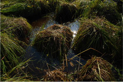
Figure A.1. Sedge fen with tussocks 'Biaza' (26 July 2011).
Download figure:
Standard image High-resolution image
Figure A.2. Birch-dominated poor fen 'Chuvashi' (date of photo—24 July 2011).
Download figure:
Standard image High-resolution image
Appendix B.: Methane flux measurements
The air inside of the chamber was circulated by a battery-operated internal fan; a water channel on the chamber rim acted as a lock against leaks into or out of the chamber. The bottom of the collar was inserted into the soil at the depth of 10 cm at the time of about 15 min before the start of the measurements. Gas was sampled in equal intervals at the times t0 = 0, t1, t2 and t3 into nylon syringes ('SFM', Germany). The total measurement time (Δt = t3 − t0) was chosen according to the ecosystem type and varied from 21 to 60 min on the sites with a probably high and low fluxes respectively. Syringes were sealed by rubber stoppers and delivered to the laboratory.
Methane concentrations were measured by a gas chromatograph 'Crystal-5000' ('Chromatec' Co., Ioshkar-Ola, Russia) with an FID and column (3 m) filled by HayeSep Q (80–100 mesh) at 70 °C with nitrogen as a carrier gas (flow rate 30 ml min−1). These measured concentrations were corrected based on a test experiment of leakage from the syringes between sampling and measurement, which found that an initial CH4 concentration of 5 ppm decreased with the rate of 0.02% per hour.
Appendix C.: CH4 emission from subtaiga fen and poor fen of Western Siberia
See table C.1.
Table C.1. CH4 emission from subtaiga fen and poor fen of Western Siberia.
| Coordinates | CH4 fluxes (mgC m−2 h−1) | |||||||
|---|---|---|---|---|---|---|---|---|
| Point number | Latitude | Longitude | Date | WTL (cm)a | pH | The most abundant speciesb | Mean | STDc |
| Subtaiga, Birch poor fen, 2011 | ||||||||
| 1 | 56.413 05 | 78.796 71 | 9.07 | −16 | 4.9 | Men, Com, Fal | 1.08 | 0.05 |
| 0.95 | 0.23 | |||||||
| 0.90 | 0.04 | |||||||
| 2 | 56.413 03 | 78.796 68 | 9.07 | −18 | 4.9 | Men, Com, Fal | 0.64 | 0.06 |
| 0.74 | 0.01 | |||||||
| 0.47 | 0.03 | |||||||
| 3 | 56.413 05 | 78.796 75 | 9.07 | −22 | 4.8 | And, Nan, Fal | 0.40 | 0.02 |
| 0.50 | 0.03 | |||||||
| 0.31 | 0.06 | |||||||
| 4 | 56.413 05 | 78.796 75 | 9.07 | −14 | 4.7 | Men, Com, Sch | 0.67 | 0.06 |
| 0.57 | 0.04 | |||||||
| 0.72 | 0.03 | |||||||
| 5 | 56.413 05 | 78.796 75 | 9.07 | −15 | 4.7 | Men, Com, Sch | 0.85 | 0.03 |
| 0.87 | 0.03 | |||||||
| 1.01 | 0.03 | |||||||
| 6 | 56.413 05 | 78.796 75 | 9.07 | −14 | 4.7 | Com, Men, Sch | 0.66 | 0.11 |
| 0.52 | 0.04 | |||||||
| 0.49 | 0.05 | |||||||
| 7 | 56.422 05 | 78.794 05 | 10.07 | 1 | 5.3 | Men, Com, Fal | 2.01 | 0.08 |
| 2.10 | 0.14 | |||||||
| 2.21 | 0.05 | |||||||
| 8 | 56.422 05 | 78.794 05 | 10.07 | 3 | 5.3 | Men, Eqf, Fal | 2.26 | 0.06 |
| 2.43 | 0.14 | |||||||
| 2.55 | 0.10 | |||||||
| 9 | 56.422 05 | 78.794 05 | 10.07 | 1 | 5.3 | Men, Com, Eqf | 1.79 | 0.06 |
| 1.92 | 0.12 | |||||||
| 1.86 | 0.14 | |||||||
| 10 | 56.422 01 | 78.794 01 | 10.07 | −18 | 5.1 | And, Nan, Fal | 0.33 | 0.07 |
| 0.29 | 0.01 | |||||||
| 0.41 | 0.07 | |||||||
| 11 | 56.422 01 | 78.794 01 | 10.07 | −20 | 5.1 | And, Nan, Fal | 0.57 | 0.05 |
| 0.52 | 0.04 | |||||||
| 0.51 | 0.06 | |||||||
| 12 | 56.422 01 | 78.794 01 | 10.07 | −23 | 5.1 | And, Nan, Fal | 0.29 | 0.01 |
| 0.18 | 0.02 | |||||||
| 0.21 | 0.03 | |||||||
| 13 | 56.422 01 | 78.793 98 | 11.07 | −10 | 5.1 | Sch, Com, Fal | 0.92 | 0.06 |
| 1.01 | 0.05 | |||||||
| 0.87 | 0.05 | |||||||
| 14 | 56.422 01 | 78.793 96 | 11.07 | −1 | 5.1 | Sch, Com Fal | 1.78 | 0.05 |
| 1.84 | 0.06 | |||||||
| 1.74 | 0.06 | |||||||
| 15 | 56.422 02 | 78.793 95 | 11.07 | 0 | 5.1 | Men, Com. Sch | 1.91 | 0.04 |
| 1.74 | 0.04 | |||||||
| 2.03 | 0.05 | |||||||
| 16 | 56.422 00 | 78.793 89 | 11.07 | −10 | 5.8 | Men, Sch, Fal | 1.07 | 0.08 |
| 0.98 | 0.13 | |||||||
| 1.20 | 0.08 | |||||||
| 17 | 56.422 01 | 78.793 91 | 11.07 | −2 | 6.6 | Men, Com, Eqf | 1.54 | 0.11 |
| 1.78 | 0.08 | |||||||
| 1.90 | 0.15 | |||||||
| 18 | 56.422 01 | 78.793 92 | 11.07 | 1 | 6.6 | Men, Com, Eqf | 1.41 | 0.08 |
| 1.72 | 0.15 | |||||||
| 1.76 | 0.08 | |||||||
| Subtaiga, Reed cane-sedge fen, 2011 | ||||||||
| 19 | 56.500 42 | 78.311 85 | 12.7 | 0 | 6.4 | Ces, Com, Phr | 2.21 | 0.17 |
| 2.04 | 0.17 | |||||||
| 2.17 | 0.24 | |||||||
| 20 | 56.500 42 | 78.311 85 | 12.7 | −2 | 6.4 | Ces, Com, Phr | 2.37 | 0.23 |
| 2.42 | 0.16 | |||||||
| 2.59 | 0.30 | |||||||
| 21 | 56.500 42 | 78.311 85 | 12.7 | 1 | 6.4 | Ces, Com, Phr | 1.70 | 0.13 |
| 1.90 | 0.27 | |||||||
| 1.87 | 0.13 | |||||||
| 22 | 56.500 42 | 78.311 85 | 26.7 | 10 | 6.3 | Ces, Com, Phr | 3.08 | 0.76 |
| 2.84 | 0.10 | |||||||
| 2.94 | 0.09 | |||||||
| 23 | 56.500 42 | 78.311 85 | 26.7 | 7 | 6.3 | Ces, Com, Phr | 2.54 | 0.21 |
| 3.01 | 0.20 | |||||||
| 2.71 | 0.13 | |||||||
| 24 | 56.500 42 | 78.311 85 | 26.7 | −12.5 | 6.3 | Ces, Com, Phr | 0.73 | 0.36 |
| 0.86 | 0.09 | |||||||
| 1.28 | 0.38 | |||||||
| 25 | 56.500 42 | 78.311 85 | 26.7 | 6 | 6.3 | Ces, Com, Phr | 1.61 | 0.31 |
| 1.49 | 0.12 | |||||||
| 1.61 | 0.26 | |||||||
| 26 | 56.500 42 | 78.311 85 | 26.7 | −1 | 6.3 | Ces, Com, Phr | 1.07 | 0.20 |
| 1.23 | 0.16 | |||||||
| 1.01 | 0.18 | |||||||
| 27 | 56.500 42 | 78.311 85 | 26.7 | 5 | 6.3 | Ces, Com, Phr | 2.26 | 0.43 |
| 2.54 | 0.10 | |||||||
| 2.34 | 0.32 | |||||||
| Subtaiga, Birch poor fen, 2011 | ||||||||
| 28 | 56.411 45 | 78.797 12 | 27.7 | −9 | 5.2 | Men, Com, Sch | 0.65 | 0.23 |
| 0.71 | 0.08 | |||||||
| 0.86 | 0.23 | |||||||
| 29 | 56.411 45 | 78.797 12 | 27.7 | −11 | 5.2 | Men, Com, Sch | 0.98 | 0.10 |
| 0.95 | 0.12 | |||||||
| 1.14 | 0.06 | |||||||
| 30 | 56.411 45 | 78.797 12 | 27.7 | −12 | 5.2 | Com, Men, Sch | 1.07 | 0.04 |
| 1.23 | 0.17 | |||||||
| 1.03 | 0.18 | |||||||
| 32 | 56.411 46 | 78.797 17 | 27.7 | −12 | 5.2 | Men, Com, Sch | 1.12 | 0.07 |
| 0.99 | 0.13 | |||||||
| 1.12 | 0.24 | |||||||
| 33 | 56.411 46 | 78.797 17 | 27.7 | −7 | 5.2 | Men, Com, Sch | 1.31 | 0.07 |
| 1.28 | 0.23 | |||||||
| 1.23 | 0.11 | |||||||
| 34 | 56.411 46 | 78.797 17 | 27.7 | −8 | 5.2 | Com, Men, Sch | 1.50 | 0.19 |
| 1.38 | 0.20 | |||||||
| 1.55 | 0.28 | |||||||
| 35 | 56.411 41 | 78.797 26 | 27.7 | −15 | 5.0 | And, Nan, Fal | 0.82 | 0.16 |
| 0.78 | 0.03 | |||||||
| 0.67 | 0.02 | |||||||
| 36 | 56.411 41 | 78.797 26 | 27.7 | −13 | 5.0 | And, Nan, Fal | 0.66 | 0.03 |
| 0.73 | 0.03 | |||||||
| 0.85 | 0.22 | |||||||
| 37 | 56.411 41 | 78.797 26 | 27.7 | −16 | 5.0 | And, Nan, Fal | 0.97 | 0.08 |
| 0.94 | 0.10 | |||||||
| 0.89 | 0.03 | |||||||
| Subtaiga, Reed cane-sedge fen, 2011 | ||||||||
| 38 | 56.500 36 | 78.311 80 | 28.7 | −4 | 6.3 | Ces, Com, Phr | 2.64 | 0.06 |
| 2.40 | 0.07 | |||||||
| 2.34 | 0.03 | |||||||
| 39 | 56.500 36 | 78.311 80 | 28.7 | −6 | 6.3 | Ces, Com, Phr | 1.65 | 0.18 |
| 1.57 | 0.07 | |||||||
| 1.49 | 0.05 | |||||||
| 40 | 56.500 36 | 78.311 80 | 28.7 | 5 | 6.3 | Ces, Com, Phr | 3.07 | 0.07 |
| 2.77 | 0.19 | |||||||
| 2.87 | 0.03 | |||||||
| 41 | 56.500 33 | 78.311 78 | 28.7 | 10 | 6.3 | Ces, Com, Phr | 2.22 | 0.24 |
| 2.49 | 0.76 | |||||||
| 2.67 | 0.11 | |||||||
| 42 | 56.500 33 | 78.311 78 | 28.7 | 5 | 6.3 | Ces, Com, Phr | 2.17 | 0.30 |
| 2.38 | 0.21 | |||||||
| 2.30 | 0.08 | |||||||
| 43 | 56.500 33 | 78.311 78 | 28.7 | 12 | 6.3 | Ces, Com, Phr | 3.32 | 0.13 |
| 3.18 | 0.36 | |||||||
| 3.02 | 1.30 | |||||||
| 44 | 56.500 33 | 78.311 87 | 20.8 | 5 | 6.1 | Ces, Com, Phr | 2.79 | 0.13 |
| 3.10 | 0.12 | |||||||
| 2.48 | 0.17 | |||||||
| 2.15 | 0.28 | |||||||
| 45 | 56.500 33 | 78.311 88 | 20.8 | 6 | 6.1 | Ces, Com, Phr | 2.47 | 0.27 |
| 2.80 | 0.12 | |||||||
| 3.02 | 0.23 | |||||||
| 2.38 | 0.27 | |||||||
| 46 | 56.500 34 | 78.311 87 | 20.8 | 5 | 6.1 | Act, Com, Phr | 2.81 | 0.10 |
| 2.60 | 0.14 | |||||||
| 2.07 | 0.02 | |||||||
| 47 | 56.500 32 | 78.311 90 | 20.8 | 7 | 6.1 | Act, Com, Phr | 3.14 | 0.12 |
| 2.83 | 0.14 | |||||||
| 2.28 | 0.06 | |||||||
| 48 | 18.715 80 | 56.500 30 | 20.8 | 5 | 6.1 | Act, Com, Phr | 2.26 | 0.08 |
| 2.74 | 0.10 | |||||||
| 2.95 | 0.03 | |||||||
| 49 | 18.717 60 | 56.500 28 | 20.8 | 8 | 6.1 | Act, Com, Phr | 2.13 | 0.04 |
| 3.36 | 0.05 | |||||||
| 2.54 | 0.02 | |||||||
| Subtaiga, Birch poor fen, 2011 | ||||||||
| 50 | 56.413 05 | 78.796 71 | 21.8 | −17 | 5.3 | Men, Com, Fal | 1.62 | 0.03 |
| 1.72 | 0.16 | |||||||
| 2.02 | 0.04 | |||||||
| 51 | 56.413 03 | 78.796 68 | 21.8 | −11 | 5.3 | Men, Com, Fal | 1.01 | 0.06 |
| 1.27 | 0.07 | |||||||
| 0.83 | 0.07 | |||||||
| 52 | 56.413 01 | 78.796 65 | 21.8 | −16 | 5.3 | Men, Com, Fal | 1.52 | 0.08 |
| 1.32 | 0.05 | |||||||
| 1.16 | 0.02 | |||||||
| 53 | 56.412 99 | 78.796 62 | 21.8 | −16 | 5.3 | Men, Com, Fal | 1.00 | 0.07 |
| 0.94 | 0.03 | |||||||
| 0.74 | 0.10 | |||||||
| 54 | 56.412 97 | 78.796 59 | 21.8 | −6 | 5.6 | Men, Fal | 2.01 | 0.20 |
| 1.82 | 0.08 | |||||||
| 2.42 | 0.13 | |||||||
| 55 | 56.412 95 | 78.796 56 | 21.8 | −16 | 5.6 | Men, Chm, Fal | 0.91 | 0.12 |
| 0.81 | 0.05 | |||||||
| 0.72 | 0.09 | |||||||
aPositive or negative values of WTL (water table level) correspond to situations when WTL is lower or higher than the mean level of mosses, respectively. bAct—Carex acuta; And—Andromeda polifolia; Ces—Carex cespitosa;Chm—Chamaedaphne calyculata; Com—Comarum palustre; Eqf—Equisetum fluviatile; Fal—Sphagnum fallax; Men—Menyanthes trifoliata; Nan—Betula nana;Phr—Phragmites australis; Sch—Scheuchzeria palustris. cStandard deviation of flux value given from propagation of uncertainty using the parameter errors through the linear regression.