

Abstract
Recent investments in the transit sector to address greenhouse gas emissions have concentrated on purchasing efficient replacement vehicles and inducing mode shift from the private automobile. There has been little focus on the potential of network and operational improvements, such as changes in headways, route spacing, and stop spacing, to reduce transit emissions. Most models of transit system design consider user and agency cost while ignoring emissions and the potential environmental benefit of operational improvements. We use a model to evaluate the user and agency costs as well as greenhouse gas benefit of design and operational improvements to transit systems. We examine how the operational characteristics of urban transit systems affect both costs and greenhouse gas emissions. The research identifies the Pareto frontier for designing an idealized transit network. Modes considered include bus, bus rapid transit (BRT), light rail transit (LRT), and metro (heavy) rail, with cost and emissions parameters appropriate for the United States. Passenger demand follows a many-to-many travel pattern with uniformly distributed origins and destinations. The approaches described could be used to optimize the network design of existing bus service or help to select a mode and design attributes for a new transit system. The results show that BRT provides the lowest cost but not the lowest emissions for our large city scenarios. Bus and LRT systems have low costs and the lowest emissions for our small city scenarios. Relatively large reductions in emissions from the cost-optimal system can be achieved with only minor increases in user travel time.
Export citation and abstract BibTeX RIS

Content from this work may be used under the terms of the Creative Commons Attribution 3.0 licence. Any further distribution of this work must maintain attribution to the author(s) and the title of the work, journal citation and DOI.
1. Introduction
In the United States, the public transportation sector emitted approximately 14 million metric tons of carbon dioxide in 2011 (FTA 2013, US EIA 2013, EPA 2004, Carbon Trust 2013). Recent investments in this sector to address greenhouse gas (GHG) emissions have concentrated on purchasing efficient replacement vehicles and inducing mode shift from the private automobile (Gallivan and Grant 2010). However, there has been little focus on the potential of operational improvements to reduce transit emissions. It is known that increasing stop spacing can reduce bus emissions (Saka 2003), but there are many other operational and network design improvements that have not been considered. Examining a city transit network, there is the potential to reduce both costs and emissions by improving system efficiency. This letter examines the extent to which system characteristics (i.e., headway, route spacing, and stop spacing) and trunk technology (i.e., heavy rail light rail, and bus) can be modified to reduce GHG emissions and user and agency costs. The research employs continuum approximation models to design a grid transit network for GHG emissions and social cost minimization. The objective is to evaluate the potential benefit of design and operational approaches to improving the environmental efficiency of transit systems.
This letter focuses on the network design and operation of transit systems with fixed ridership. Demand is considered exogenous, and a grid network is considered for simplicity. Decision variables include headway, stop spacing, and route spacing. We consider different trunk line technologies: metro (heavy) rail, light rail transit (LRT), bus rapid transit (BRT), and bus. The environmental metric is life-cycle GHG emissions. The scope of the life-cycle emissions and costs includes infrastructure construction, system maintenance, and vehicle manufacturing and operations. Although a metric of energy would help avoid an assumption of electricity mix, GHG emissions provide a more direct measure of the environmental impact. Other environmental emissions, particularly criteria air pollutants, are outside the scope of this letter.
2. Literature review
The literature review begins with a discussion of public transportation emissions inventories, approaches to reducing emissions, and how those emissions are affected by transit operations. The second part describes models for optimizing transit operations.
2.1. Emissions from public transportation
Many studies have attempted to quantify or compare the emissions from buses (Herndon et al 2005, Puchalsky 2005, Ally and Pryor 2007, Chester and Horvath 2009, Cui et al 2010) and rail transit (Puchalsky 2005, Messa 2006, Chester and Horvath 2009, Chester et al 2013), but fewer have attempted to examine the life-cycle beyond the operations phase (Ally and Pryor 2007, Chester and Horvath 2009, Chester et al 2010, Cui et al 2010). This discrepancy may be due to a greater policy focus on tailpipe emissions. As well, estimating the environmental effects of infrastructure is complicated while Puchalsky (2005) compared emissions from bus rapid transit (BRT) and light rail transit (LRT), he only examined emissions from the operation of the vehicles, omitting the significant emissions for infrastructure construction, maintenance, and operation identified by Chester and Horvath (2009). For example, the per-passenger-kilometer-travelled operating GHG emissions are comparable for peak-hour urban diesel and commuter rail, but when the rest of the life-cycle is included, the GHG emissions of commuter rail are nearly double that of bus (Chester and Horvath 2009). Furthermore, life-cycle assessment studies have generally been case studies, making it difficult to generalize results to other locations and various technologies. For example, emissions from electric rail or bus services are dependent on the local electricity mix (Messa 2006, Chester and Horvath 2009, Cooney et al 2013).
A recent Transit Cooperative Research Program report (Gallivan and Grant 2010) identifies several ways in which transit agencies are reducing GHG emissions: expanding transit service, increasing vehicle passenger loads, reducing roadway congestion, promoting compact development, alternative fuels and vehicle types, vehicle operations and maintenance, infrastructure construction and maintenance, and reducing emissions from facilities and nonrevenue vehicles. Some of these approaches, however, are not necessarily cost effective or effective at reducing emissions. The approaches can be generalized into those that reduce the emissions of the transit system (Cook and Straten 2001, Schimek 2001, Stasko and Gao 2010) and those that cause transit to displace other emission sources (Vincent and Jerram 2006, Hensher 2008, McDonnell et al 2008). Schimek (2001) found that it is more economical to retrofit diesel engines rather than buy new vehicles, while Stasko and Gao (2010) developed a model for optimizing vehicle retrofit, replacement, and assignment decisions. Reductions due to displaced emissions are difficult to estimate or forecast as they require an understanding of how mode choice may be affected by improvements in transit service. A case study of several regions in Europe found that improved transit quality attracted non-motorized users, not drivers, causing a net increase in emissions (Poudenx 2008). Emissions per passenger kilometer travelled are also highly dependent on ridership (Chester and Horvath 2009).
While Gallivan and Grant (2010) mention 'transit agency operations' in their report, their focus in that area is on the reduction of tailpipe emissions through engine upgrades and low-carbon fuels, reduction of energy consumption in facilities, and the impacts of construction and maintenance. Other operational improvements that could improve emissions include (1) increasing spacing between stops in order to increase the average vehicle speed and reduce the number of accelerations and decelerations, (2) signal priority, (3) using smaller vehicles, and (4) reducing the number of vehicles required to satisfy user demand. These approaches have not been discussed at length in the literature. In one study, an optimal bus stop spacing of 700–800 m, rather than the US average of 330 m, was found to reduce fuel consumption and carbon dioxide emissions substantially by reducing stops and starts and increasing the average speed, but had little effect on other air emissions (Saka 2003). Others have examined ways of optimizing the assignment and scheduling of 'green vehicles' within a fleet that includes older vehicles to reduce total emissions (Beltran et al 2009, Li and Head 2009). Dessouky et al (2003) jointly optimized costs, service, and emissions for a demand-responsive transit service, but a similar approach has not yet been applied to fixed-route public transportation systems Diana et al (2007) compared the emissions impacts of traditional fixed-route and demand-responsive service at different demand and services levels. Emissions were based solely on distance travelled, and analysis ignored the potential impacts of average speed, acceleration, and deceleration.
2.2. Public transportation network design
There have been numerous studies on transit system design, but very few have included any environmental metrics (Dessouky et al 2003, Saka 2003, Diana et al 2007, described above). Continuum approximation (CA) models have been used to optimize transportation network design to minimize system and user costs. These models can provide general insights into how to structure efficient transit systems by making generalizations that simplify the analysis. Several studies have used CA to optimize stop spacing (Wirasinghe and Ghoneim 1981, Kuah and Perl 1988, Parajuli and Wirasinghe 2001) along with other network attributes such as headway (Chien et al 2010). Others have examined the structure of transit networks, such as grids, radial systems (Byrne 1975, Tirachini et al 2010), and hub-and-spoke systems (Newell 1979). Tirachini et al (2010) compared light rail, heavy rail, and BRT on a radial transit network. Daganzo (2010) went a step further by determining a system design and operating characteristics that could make transit competitive with the automobile. Applying his models to Barcelona, he found that optimal service would reduce the total number of vehicles significantly, thus reducing total transit emissions. Sivakumaran et al (2013) explored the influence of access mode on choice of trunk technology, and the research in this letter builds on the models developed for that research. Continuum approximation models are a promising approach for the joint optimization of costs and emissions, having been used for cost minimization in previous research.
3. Methodology
Consider a large rectangular urban area with a dense grid road network (see figure 1). The transit network consists of two sets of many parallel lines with uniform spacing, rL and rW, travelling lengthwise and widthwise to form a grid covering the city. Stops are equidistant with spacing s, and route spacing is an integer multiple of stop spacing (rL = pLs, rW = pWs). Due to the grid structure of the network, line spacings for latitudinal lines have to be a multiple of the stop spacings on the longitudinal lines, and vice verse, so that transfers from one line to another do not incur additional walking. Headways between vehicles on each line are H. The density of trip origins is assumed to be uniform throughout the urban area, with travellers exhibiting a many-to-many demand pattern. Each user travels on foot along the grid street network to the nearest transit stop. The city can be described through several model parameters, which are explained in table 1. The transit modes include diesel bus, BRT, LRT, and metro heavy rail transit. Speed, time, cost, and emissions parameters for each mode are given in table 2. The time and speed parameters are taken from Sivakumaran et al (2013). The right-of-way (ROW) infrastructure parameters (CI, EI) include the maintenance of pavement for bus and BRT, the construction of the track for LRT and metro, and the construction of a combination of elevated, at-grade, and aerial right-of-way for metro. The station parameters (CS, ES) account for the construction of the stations, and the vehicle parameters (CV, EV) account for the acquisition, operation, and maintenance of transit vehicles. For inclusion in the model, these parameters have been normalized by appropriate units to represent the useful life. Their derivation is described in detail in the appendices (tables A.1–A.4, B.1–B.4). The BRT system is based on the proposed design for the Geary Blvd BRT, LRT is based on the Muni Metro system, and metro is based on the Bay Area Rapid Transit (BART) system, all in the San Francisco Bay Area in California. Emissions estimates were taken from Chester and Horvath (2009) and assume a California energy mix.
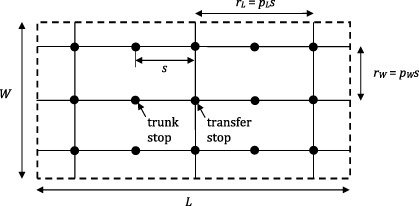
Figure 1. Rectangular city (L × W) with a grid–trunk system.
Download figure:
Standard image High-resolution imageTable 1. Model parameters for city.
| Parameter | Description | Value | Units |
|---|---|---|---|
| δ | Demand density | Varies | pax/km2-h |
| L | Length of urban area | Varies | km |
| W | Width of urban area | Varies | km |
| va | User access speed | 5 | km/h |
| μ | User value-of-time | Varies | $/h |
Table 2. Mode-specific model parameters.
| Param | Description | Units | Bus | BRT | LRT | Metro |
|---|---|---|---|---|---|---|
| v | Commercial speed | km/h | 25 | 40 | 40 | 60 |
| τ | Lost time/stop | s | 30 | 30 | 30 | 45 |
| T | Lost time/transfer | s | 20 | 30 | 30 | 60 |
| CI | ROW infrastructure cost | $/km-h | 10 | 36 | 220 | 260 |
| CV | Vehicle purchase, fuel and maintenance cost | $/veh-km | 1.0 | 1.6 | 6.0 | 8.9 |
| CM | Labor cost | $/veh-h | 150 | 200 | 200 | 250 |
| CS | Station construction cost | $/st-h | 0.82 | 8.2 | 11 | 130 |
| EI | ROW infrastructure emissions | g/km h | 8.1 | 160 | 790 | 44 000 |
| EV | Vehicle fleet manufacturing, operation and maintenance emissions | g/veh-km | 1700 | 2200 | 2700 | 11 000 |
| ES | Station construction emissions | g/st-h | 170 | 1700 | 1700 | 120 000 |
Developing analytical expressions for user cost and system emissions, we can evaluate the tradeoffs between level of service for users and environmental impacts with different values of the decision variables (see table 3). Optimal values of H, p, and s can be chosen to minimize total system cost subject to a GHG emissions constraint, which can then be varied. The total system cost is the sum of the user and agency costs, and the cost expressions were taken from Sivakumaran et al (2013). User cost (Zuser) is made up of the sum of the:
- expected access and egress time,
 ,
, - wait time, ,
- transfer time, ,
- and vehicle travel time,


multiplied by the total demand, D = δLW, and wage rate, μ. Wage rate serves as a proxy for value-of-time. Agency cost (Zagency) is driven by:
- the total infrastructure length of the system, ,
- the number of stations in the system, ,
- the total vehicular distance travelled by transit vehicles in an hour of operation, ,
- and the vehicle fleet size, .


Using these expressions, the system cost function (Zsystem) is given by:
Table 3. Decision variables.
| Decision variable | Description | Units |
|---|---|---|
| H | Transit vehicle headway | h |
| p | Route spacing factor | km |
| s | Stop spacing | km |
GHG emissions are measured in carbon dioxide equivalents, a metric that normalizes all GHG emissions to the equivalent mass of CO2. The total operating GHG emissions per year, Zemissions, is based on the system emissions because there are negligible emissions for the user when the access mode is walking. The formulation is identical to the agency cost expression, except that the term corresponding to labor cost is removed because there is not an emissions equivalent:
This constrained optimization involves conflicting objectives which can be displayed using Pareto curves. Using the above models and the associated parameters, we can solve for the values of the decision variables that minimize the total system costs subject to an emissions constraint:
where E is a GHG emissions constraint. By varying E, we can develop a set of optimal system characteristics, H*, p*, s*, for given emissions goals. These Pareto curves are bound at one end by the system cost-optimal point where increases to E will provide no additional cost reductions. The other end of the curve is unbounded.
Once an optimal system is obtained, we can observe the behavior of the cost and emission models. For example, figure 2 shows optimal system, user, and agency cost curves for a bus system as the GHG emission constraint varies. The vertical bar at the right of the curve marks the system cost-optimal point, where further increases in emissions will not reduce the costs. Agency costs increase with emissions while user costs decrease with emissions. The agency costs decrease when emissions are constrained because emissions reductions are caused by reductions in service. Excessive reductions in service levels may cause riders to abandon public transit for other, more polluting, modes. User costs can rise significantly when emission reductions are steep, as shown at the extreme left of the graph in figure 2.

Figure 2. System, user, and agency costs for a bus system by GHG emissions level.
Download figure:
Standard image High-resolution image4. Results and discussion
The Pareto curves of optimal system cost and emissions can be used in several ways to inform transit system design. The slope of a tangent on the Pareto curve is the shadow price at the tangent point, or the cost of reducing emissions by an additional unit. This curve can be used to determine how much to reduce emissions by finding the point at which the shadow price is equal to the market carbon price. That point indicates the economically efficient combination of cost and GHG emissions (see figure 2). At that point, the cost of reducing an additional unit of emissions would be greater than the price of carbon on the market. An example of the carbon price analysis is described in section 4.25.
The optimal system design depends largely on the type of city for which the system is being designed. Section 4.1 presents the results of parametric analysis of the three model parameters that describe city characteristics, city size (L,W), demand density (δ), and wage rate (μ). Since demand density and wage rate appear as a product in a single term (μD = μδLW) in the cost expression, it is meaningless to vary them individually. Hereon, we will refer to the product of μ and δ as β. We consider small (L = W = 10 km) and large (L = W = 40 km) city sizes, low passenger demand densities (δ = 100 pax/km2/h) and wage rates (μ = $10/h) (β = $1000 − pax/km2/h2), and high passenger demand densities (δ = 200 pax/km2/h) and wages (μ = $20/h) (β = $4000-pax/km2/h). The parameter values were chosen for hypothetical cities and do not necessarily reflect standard definitions of low and high values for the city characteristics. They combine into four possible city scenarios, described in table 4.
Table 4. City scenarios.
| City size (L,W) (km) | Demand density (δ) (pax/km2/h) | Wage rate (μ ) ($/h) | β = μδ ($-pax/km2/ h2) | |||||
|---|---|---|---|---|---|---|---|---|
| Scenario 1 | Small | 10 | Low | 100 | Low | 10 | Low | 1000 |
| Scenario 2 | Small | 10 | High | 200 | High | 20 | High | 4000 |
| Scenario 3 | Large | 40 | Low | 100 | Low | 10 | Low | 1000 |
| Scenario 4 | Large | 40 | High | 200 | High | 20 | High | 4000 |
The hypothetical cities in the parametric analysis do not represent actual cities, but the relative characteristics do resemble some real US cities. For example, scenario 1 is similar to Fresno, California, scenario 2 to San Francisco, scenario 3 to Kansas City, Missouri, and scenario 4 to New York City or Chicago.
4.1. Parametric analysis
Beginning with pair-wise analysis of the four city scenarios, we can observe the system changes that occur when β is changed. Figure 3 shows the Pareto frontiers for optimal transit system design by mode for a small city with low (scenario 1) and high values of β (scenario 2). For scenario 1, BRT is just barely the lowest cost option for most values of the GHG emissions constraint. At the cost-optimal point at the right end of the curve, however, bus and LRT have lower emissions than BRT. Metro is not competitive in this scenario as its costs are higher than both bus and BRT and its emissions at the cost-optimal point are at least four times that of the other modes. The attributes of the systems at the cost-optimal point (shown in table 5) reveal how the mode parameters impact the relative costs and emissions. The low infrastructure cost of bus allows for small stop (s = 0.8 km) and route (ps = 1.6 km) spacing compared to the other modes, which have route spacing between 1.8 and 3.6 km. The small spacings for bus make access on foot easier, and thus keep the out-of-vehicle travel time much lower (14 min, or 58% lower than metro). This result regarding route spacing is consistent with the findings of Tirachini et al (2010). BRT, which is faster than bus, has a slight edge in system cost because the travel time is 5 min shorter. LRT is able to be competitive for emissions because it has cost-optimal route spacing 50% higher than bus or BRT, so the amount of required infrastructure and number of vehicles in operation are lower. The emissions results in tables 5 and 6 are shown to no more than two significant digits because the quality of the data and the accuracy of the model do not justify greater precision. The section on sensitivity analysis provides further explanation.
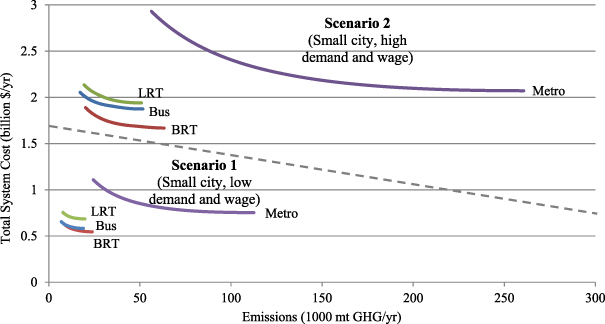
Figure 3. Pareto frontiers of optimal transit system design for a small city (L = W = 10 km) for bus, BRT, LRT, and metro.
Download figure:
Standard image High-resolution imageTable 5. Cost-optimal decision variables, costs, emissions, and average travel time (TT) for a small city. (Note: OVTT—out-of-vehicle travel time.)
| p | s (km) | H (min) | Zsystem (billion $) | GHG (1000 mt) | TT (min) | OVTT (min) | |
|---|---|---|---|---|---|---|---|
| Scenario 1 | (Small city, low demand and wage) | ||||||
| Bus | 2 | 0.8 | 9 | 0.6 | 19 | 44 | 24 |
| BRT | 2 | 0.9 | 8 | 0.5 | 25 | 39 | 25 |
| LRT | 3 | 1.0 | 8 | 0.7 | 20 | 45 | 31 |
| Metro | 3 | 1.2 | 8 | 0.8 | 110 | 49 | 38 |
| Scenario 2 | (Small city, high demand and wage) | ||||||
| Bus | 1 | 0.9 | 6 | 1.9 | 52 | 37 | 17 |
| BRT | 1 | 1.0 | 6 | 1.7 | 67 | 31 | 18 |
| LRT | 2 | 0.8 | 5 | 1.9 | 51 | 35 | 21 |
| Metro | 2 | 1.0 | 5 | 2.1 | 260 | 36 | 25 |
When β is quadrupled (figure 3—scenario 2), the costs and emissions increase for all modes. With the increase in value-of-time for users, the agency must improve service to minimize the system cost. The cost-optimal route spacings for bus and BRT are cut nearly in half and the route spacings for the other modes are also reduced. Along with the decrease in headways, the service improvements lead to a reduction in travel time for users at the cost-optimal point. While bus and LRT have lower cost-optimal emissions, BRT service has a lower cost and a greater travel time advantage than in the low β scenario.
Comparison of the remaining scenarios (figure 4) reveals similar patterns between low and corresponding high β cities. Additionally, we observe that, with an increase in β, bus systems have significant loss in cost advantage relative to the other modes. In the large cities the benefit of short access distances for bus is outweighed by the disbenefit of the slow speed and many stops that increase the travel time. Improved service is required to balance the increased impact of user costs as the number of users and their wages increase, and this service increases both the agency costs and emissions. As shown in table 6, the service improvements help to reduce the travel time for users compared to the low β cities (scenarios 1 and 3), by reducing headways and route spacing. Bus has the greatest headway reductions, the smallest route spacing reductions, and the smallest travel time reductions. The route and stop spacings appear to be as low as they can optimally be because of the tradeoff between access time and stop time in the vehicle. For metro we see travel time reductions of up to 20% as route spacing and headway reductions reduce out-of-vehicle time without increasing in-vehicle travel time. Scenario 4, which most resembles a high-density metropolis, is the only case where metro has the lowest travel time, but BRT still has a slight cost advantage that, however, may not be significant. We expect that the addition of bus feeder service will provide additional advantages to BRT, LRT and metro for larger, higher-density cities. With faster access to stations, the fast trunk modes can operate with larger stops spacings, thus reducing user in-vehicle travel time and agency costs (Sivakumaran et al 2013).
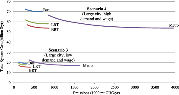
Figure 4. Pareto frontiers of optimal transit system design for a large city (L = W = 40 km) for bus, BRT, LRT, and metro.
Download figure:
Standard image High-resolution imageTable 6. Cost-optimal decision variables, costs, emissions, and average travel time (TT) for a large city. (Note: OVTT—out-of-vehicle travel time).
| p | s (km) | H (min) | Zsystem (billion $) | GHG (1000 mt) | TT (min) | OVTT (min) | |
|---|---|---|---|---|---|---|---|
| Scenario 3 | (Large city, low demand and wage) | ||||||
| Bus | 1 | 1.6 | 8 | 19 | 330 | 100 | 28 |
| BRT | 1 | 1.7 | 8 | 15 | 420 | 77 | 29 |
| LRT | 2 | 1.5 | 8 | 18 | 310 | 84 | 35 |
| Metro | 2 | 1.8 | 8 | 17 | 1600 | 79 | 41 |
| Scenario 4 | (Large city, high demand and wage) | ||||||
| Bus | 1 | 1.3 | 5 | 70 | 700 | 95 | 21 |
| BRT | 1 | 1.4 | 5 | 54 | 920 | 71 | 21 |
| LRT | 1 | 1.6 | 5 | 58 | 850 | 73 | 25 |
| Metro | 1 | 1.9 | 5 | 54 | 4000 | 66 | 29 |
Increasing the city size brings about a different set of system changes. The average travel distance is increased, and thus the in-vehicle travel time takes up a greater proportion of the trip. The costs and emissions increase by an order of magnitude because of the larger coverage area for service. Between scenarios 1 and 3, the cost-optimal route spacing and headways are relatively stable, but the stop spacing nearly doubles (table 6). This change increases the access time on foot, but also reduces the in-vehicle travel time by reducing the number of stops the vehicle makes. As the optimal results show, there is little benefit to the system in reducing headways, which remain around 8 or 9 min for all modes in scenarios 1 and 3. Decreasing headways for the large city scenarios would decrease travel times by up to 10% in the extreme case, but the extra vehicle costs and emissions would be prohibitive. BRT is the optimal system for both costs and is competitive for emissions in both large city scenarios (scenarios 3 and 4). The large cities require greater infrastructure mileage to serve the area, as well as higher speeds to reduce the travel times. BRT has the benefit of lower infrastructure costs than LRT and metro, which allows for greater coverage at a low cost, and higher speed than bus, which makes up for the slightly longer access time. Regardless, many of the emissions results are significantly different (> ± 10%) when compared using one significant digit.
The results of the parametric analysis suggest that a BRT system could be the best low-emissions option for many types of cities, and is also the lowest cost option. Bus is a low cost option in small cities, but BRT is lower cost when the wage rate and demand density are high. The optimal system attributes (p, s, H) vary between city types, so it is important that the analysis be repeated with the parameters of a specific city before a new system is designed. Metro, although cost competitive in the large cities, has emissions on the order of four times greater than any of the other modes for all scenarios. The emissions parameters used for metro, which were based on the BART system in the San Francisco Bay Area, were about an order of magnitude higher than any of the other modes. Modeling after a different metro system could potentially produce more favorable GHG emissions results.
4.2. Carbon price analysis
Another way to present the optimization results is to show the change in travel time (including both in- and out-of-vehicle travel time) and GHG emissions as the carbon price is increased relative to the cost-optimal point on the Pareto frontier, where an optimal agency would operate. This carbon price analysis of optimal transit systems allows us to determine the economically efficient level of GHG reduction. By operating at the point on the curve where the shadow price is equal to the carbon price, the system can avoid investing more than the market value in achieving additional GHG reductions. As an example here, we look at scenario 2 and examine the changes that occur as the price of carbon is increased. In figure 5, the dashed lines show the percentage change in GHG emissions as the carbon price increases, and the solid lines show the percentage change in travel time with increase in carbon price. The vertical jog in the lines for some modes shows the point where the optimal route spacing multiplier increases by one. With the large increase in route spacing, the emissions are reduced slightly more, but the travel time for users increases significantly. In general, the GHG emissions reduce more quickly than the travel times increase. Bus has the smallest reductions in emissions, while BRT has the smallest increases in the travel time for the range of carbon prices. Figure 5 shows carbon prices up to $3000, much higher than seen in the literature ($5-$65, IWGSCC 2010; $115, Knittel and Sandler 2011), but which corresponds to a travel time increase of less than 10% for LRT. For a carbon price of $100/mt, the potential emissions reductions are at most 3% and the corresponding travel time increase is negligible (less than a minute) because the cost increase is spread among many users in the system. Similarly, for a carbon price of $30/mt, the potential emissions reductions are at most 1% and the travel time increase is even smaller. Achieving these small reductions in emissions will cause almost imperceptible service changes to the system. This result suggests that greater GHG emissions reductions beyond a realistic market value of carbon could be implemented without inducing users to shift to other modes.
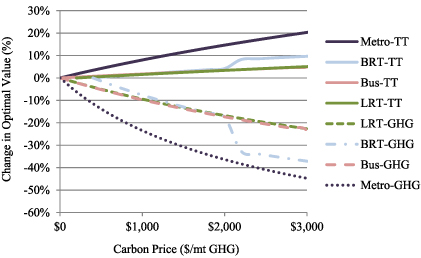
Figure 5. Change in GHG emissions and travel time with carbon price.
Download figure:
Standard image High-resolution image4.3. Sensitivity analysis
The carbon price analysis demonstrates that small changes in the values of the decision variables have a very small effect on the optimal cost, but a larger effect on the optimal emissions. To further examine this behavior of the model, we performed sensitivity analysis on the emissions parameters for BRT and metro for scenario 2. Increasing or decreasing each parameter by 50% caused small changes in the optimal cost results and produced the cost-optimal GHG emissions shown in table 7. For BRT, which requires little infrastructure investment relative to rail, changing the vehicle operations parameter (EV) was the only change to cause greater than 5% changes in the total emissions at the cost-optimal point. The changes for metro were larger (up to 15%) for the two infrastructure parameters (EI, ES).
Table 7. Sensitivity analysis on emissions parameters for cost-optimal BRT and metro for scenario 2.
| Parameter | Pct. Change | GHG (1000 mt yr−1) | |
|---|---|---|---|
| BRT | Metro | ||
| Base case | 66 | 261 | |
| EI | +50% | 67 | 275 |
| EI | −50% | 65 | 246 |
| EV | +50% | 98 | 340 |
| EV | −50% | 33 | 181 |
| ES | +50% | 68 | 298 |
| ES | −50% | 66 | 224 |
Table 8. Source of cost-optimal emissions by mode.
| Total GHG (1000 mt yr−1) | Operating and fleet (%) | ROW infrastructure (%) | Station infrastructure (%) | |
|---|---|---|---|---|
| Bus | 0.61 | 99 | 0.02 | 0.5 |
| BRT | 0.52 | 98 | 0.3 | 1.8 |
| LRT | 0.58 | 95 | 1.2 | 3.3 |
| Metro | 0.61 | 71 | 13 | 17 |
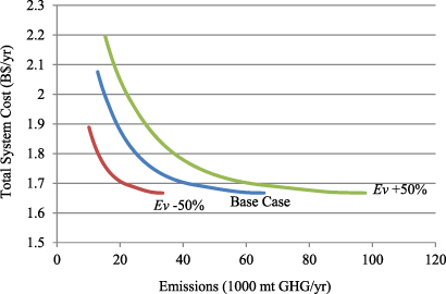
Although the optimal costs do not change with the sensitivity analysis, the emissions change with variation in EV and cause significant changes to the shape of the Pareto curve (figure 6). This result suggests that improved bus technology, such as natural gas vehicles, could significantly improve the emissions for both bus and BRT. Additionally, the operating emissions for LRT and metro are highly dependent on the electricity mix, which is the Bay Area mix for the parameters used here. A transit system in Seattle, Washington would have lower operating emissions because of the large percentage of electricity coming from hydroelectric power. Since 2009, Muni and BART have switched to cleaner energy, including 100% hydroelectric power for Muni, which would lower GHG emissions by about 60% relative to the Bay Area electricity mix used in the calculations of emissions factors in Chester and Horvath (2009), Chester (2013). In Cleveland, Ohio, on the other hand, the electricity mix is more heavily dependent on coal power, so operating emissions would be significantly higher. Examining the source of the emissions for each mode (table 8), we see that infrastructure is the source of 30% of the emissions for metro, and no more than 4.5% for the other modes. This result further emphasizes the importance of vehicle technology and electricity mix for reducing transit emissions. Additionally, our scope is limited to GHG emissions, but there are additional tradeoffs when local criteria pollutants are considered. Electric vehicles have the advantage of keeping the emissions away from the transit users, but may disproportionately affect the vulnerable population that is located near the power source (Lobscheid et al 2012).
Figure 6. Sensitivity analysis on EV for BRT.
Download figure:
Standard image High-resolution image
The emissions results are uncertain, as demonstrated by the sensitivity analysis. The final emissions can vary by as much as 50% within reasonable ranges of parameter values. The vehicle operation parameters are based on outputs from Chester and Horvath (2009), who assessed them as being of relatively good quality. They based bus operating emissions, however, on a standard drive cycle, which cannot account for the nuance in the actual model drive cycle as the stop spacing varies. Emissions from the various transportation modes may vary based on the drive cycles these modes experience. For example, in Orange County, California, bus stop spacings will be larger than in New York City, likely resulting in better fuel economy for the buses. The BRT vehicle manufacturing and operating emissions are prorated from standard diesel bus emissions, and are therefore, less accurate. Infrastructure emissions are less certain than the vehicle emissions as they are based on US industry averages from EIO-LCA (CMU 2008) and do not account for local variations. The infrastructure emissions also have a much smaller impact on the total emissions, so variation in the parameter values will have a proportionately smaller impact.
5. Conclusion
This letter presents a strategic framework for incorporating GHG emissions into transit planning decisions. Using continuum approximation models, we optimize an urban transit system for costs at different emissions constraints, and obtain a Pareto frontier of optimal transit system design. Parametric analysis of different city scenarios allows us to compare the optimal system attributes for each mode in different types of cities. Additionally, the Pareto curves help us to evaluate the system changes and user impact of GHG reductions. Results of the parametric analysis suggest that a BRT system is a low cost and low-emissions transit option for many types of cities.
Choosing GHG reduction levels based on the market price of carbon has a small impact on user travel time. This suggests that future research should explore the reasonable scope of potential emissions reductions that do not induce users to shift to other modes. Incorporating variable demand into the user cost function can allow us to estimate how many users may switch to automobile travel as transit service is reduced. It is important to remember that the GHG emissions reductions analyzed here are relative to those at the cost-optimal point. However, many existing transit systems may be operating at both higher cost and emissions outside the Pareto frontier, so that a shift to the cost-optimal point would already represent significant emissions reductions. The approaches described here could be used to optimize the network design of existing bus service or help to select the mode and design attributes for a new transit system. They can also be used by transit agencies to estimate the system cost of GHG reductions. It is important to consider that there may be equity issues with applying transit service reductions to reduce GHG emissions, and that these policies should not be implemented in isolation from other efforts to reduce automobile emissions.
This study is limited to single-mode transit systems with walking access, but relative benefits of the trunk modes are expected to change when faster feeder modes are introduced (Sivakumaran et al 2013). The results reflect a single technology for each mode (i.e., diesel for bus), and consideration of other vehicle technologies may change the results. A potential direction for future work is to examine trunk–feeder transit service, other network designs, and other potential vehicle technologies. Additionally, we do not account for the capacity of the transit vehicles. The model could be improved by varying the number of cars per train and constraining the number of boardings to the vehicle capacity.
A major assumption of this research is that demand is fixed and uniformly distributed. In reality, demand varies spatially, temporally, and with level of service. These factors have been considered in previous research on cost optimization of transit using continuum approximation models (Daganzo 2010, 2012, Kocur and Hendrickson 1982, Sivakumaran et al 2013), and could be accounted for in future development of the current model. Daganzo (2010) varied the structure and density of the transit system between the core and the periphery to account for spatial variation in transit demand. When considering temporal variation in demand, it is unclear how the network attributes may change, but the headway can easily respond to changes in demand. As for variations in response to level of service, we are currently in the process of extending their framework to account for travel time elasticities.
It should be recognized that transit systems are not currently designed for minimum GHG emissions and total societal costs. Logistical efficiencies may be part of the equation, but coverage, accessibility, and mobility to particular subpopulations are often dominating drivers. Nonetheless, by making simplifying assumptions on transit network design, the nature of the tradeoffs between minimum costs and minimum GHG emissions are more transparent.
Acknowledgments
This research was funded by a grant from the University of California Transportation Center and a Dwight David Eisenhower Graduate Transportation Fellowship.
Appendix A.: Derivation of cost parameters
Table A.1. Bus costs.
| Parameter | Value | Comments |
|---|---|---|
| CI—ROW infrastructure cost | ||
| Amortized cost ($/km h) | $10 | From Sivakumaran et al (2013). Based on assumed lifetime estimate of 20 years |
| CS—station infrastructure cost | ||
| Total cost ($/st-h) | $0.82 | 10% of BRT |
| CV—vehicle purchase, fuel and maintenance cost | ||
| Vehicle lifespan (miles) | 500 000 | Chester (2008) |
| Vehicle purchase price ($) | $330 000 | 40-ft Van Hool bus purchase by AC transit in 2007 (Gammon 2008) converted to 2012 dollars |
| Amortized vehicle price ($/veh-km) | $0.41 | |
| Maintenance cost ($/veh-km) | $0.22 | $0.20 from Clark et al (2007) converted to 2012 dollars |
| Diesel fuel price ($/gal) | $4 | US EIA (2012) |
| Fuel efficiency (mpg) | 6 | Clark et al (2007) |
| Fuel cost ($/veh-mi) | $0.67 | |
| Fuel cost ($/veh-mi) | $0.41 | |
| Total cost ($/veh-km) | $1.0 | |
| CM—labor cost | ||
| # Employees per vehicle | 3 | From Wilson (2010), Pushkarev and Zupan (1972) |
| Average wage ($/h) | $20 | |
| Wage cost ($/veh-h) | $60 | |
| Labor cost ($/veh-h) | $150 | Including agency cost markup |
Table A.2. BRT costs.
| Parameter | Value | Comments |
|---|---|---|
| CI—ROW infrastructure cost | ||
| Planning horizon (years) | 40 | |
| ROW costs ($) | $132.1 million | Converted to 2012 from budget estimate for Geary Blvd BRT project (SFCTA 2007) |
| Project length (km) | 10.5 | |
| Cost per km ($/km) | $12.6 million | |
| Amortized cost ($/km-h) | $36 | |
| CS–station infrastructure cost | ||
| Planning horizon (years) | 40 | |
| Stop costs ($) | $34.3 million | Converted to 2012 from budget estimate for Geary Blvd BRT project (SFCTA 2007) |
| Number of stops | 12 | |
| Cost per stop ($/stop) | $2.86 million | |
| Amortized cost ($/st-h) | $8.2 | |
| CV—vehicle purchase, fuel and maintenance cost | ||
| Vehicle lifespan (miles) | 500 000 | Chester (2008) |
| Vehicle purchase price ($) | $590 000 | 60-ft articulated Van Hool bus purchase by AC transit in 2007 (Gammon 2008) converted to 2012 dollars |
| Amortized vehicle price ($/veh-km) | $1.17 | |
| Maintenance cost ($/veh-km) | $0.33 | $0.20 from Clark et al (2007) prorated for larger vehicle and converted to 2012 dollars |
| Diesel fuel price ($/gal) | $4 | (US EIA 2012) |
| Fuel efficiency (mpg) | 4.62 | Clark et al (2007) prorated for relative difference in consumption (Zargari and Khan 2010) |
| Fuel cost ($/veh-mi) | $0.87 | |
| Fuel cost ($/veh-km) | $0.54 | |
| Total cost ($/veh-km) | $1.6 | |
| CM—labor cost | ||
| # Employees per vehicle | 4 | From Wilson (2010) and Pushkarev and Zupan (1972) |
| Average wage ($/h) | $20 | |
| Wage cost ($/veh-h) | $80 | |
| Labor cost ($/veh-h) | $200 | Including agency cost markup |
Table A.3. LRT costs.
| Parameter | Value | Comments |
|---|---|---|
| CI—ROW infrastructure cost | ||
| Planning horizon (years) | 40 | |
| Project cost ($) | $717 million | Converted to 2012 from costs for Muni T-third light rail line (SFMTA 2012) |
| ROW costs ($) | $645 million | Assume 90% of costs go to ROW |
| Project length (km) | 8.2 | |
| Cost per km ($/km) | $78.6 million | |
| Amortized cost ($/km-h) | $220 | |
| CS—station infrastructure cost | ||
| Planning horizon (years) | 40 | |
| Station costs ($) | $71.7 million | Assume 10% of Muni T-third budget |
| Number of stations | 18 | |
| Cost per station ($/station) | $3.98 million | |
| Amortized cost ($/st-h) | $11 | |
| CV—vehicle purchase, fuel and maintenance cost | ||
| Useful life (years) | 27 | Chester (2008) |
| Annual vehicle revenue miles (miles yr−1) | 12 000 | (MTC 2012) |
| Lifetime mileage (miles) | 324 000 | |
| Vehicle purchase price ($/veh) | $2.92 million | $2 million price (Nolte 1996) converted to 2012 dollars |
| Amortized vehicle price ($/veh-km) | $5.61 | |
| Energy use of veh (kWh/veh-km) | 4.4 | Chester and Horvath (2009) |
| Cost per kWh ($/kWh) | $0.1 | US EIA (2013) |
| Operating cost ($/veh-km) | $0.44 | |
| Total cost ($/veh-km) | $6.0 | |
| CM—labor cost | ||
| # Employees per vehicle | 4 | From Wilson (2010) and Pushkarev and Zupan (1972) |
| Average wage ($/h) | $20 | |
| Wage cost ($/veh-h) | $80 | |
| Labor cost ($/veh-h) | $200 | Including agency cost markup |
Table A.4. Metro costs.
| Parameter | Value | Comments |
|---|---|---|
| CI—ROW infrastructure cost | ||
| Planning horizon (years) | 40 | |
| Project cost ($) | $1.82 billion | Converted to 2012 from costs for BART SF airport extension (FTA 2005) |
| ROW costs ($) | $1.64 billion | Assume 90% of costs go to ROW |
| System length (km) | 17.7 | |
| Cost per km ($/km) | $92.6 million | |
| Amortized cost ($/km-h) | $260 | |
| CS—station infrastructure cost | ||
| Planning horizon (years) | 40 | |
| Station costs ($) | $71.7 million | Assume 10% of SF airport extension |
| Number of stations | 4 | |
| Cost per station ($/station) | $45.5 million | |
| Amortized cost ($/st-h) | $130 | |
| CV—vehicle purchase, fuel and maintenance cost | ||
| Useful life (years) | 40 | Chester (2008) |
| Annual vehicle revenue miles (miles yr−1) | 66 000 | MTC (2012) |
| Lifetime mileage (miles) | 2 640 000 | |
| Vehicle purchase price ($/veh) | $2.92 million | Average 8.4 cars per train Chester (2008); Contract price for new BART cars (BART 2012) |
| Amortized vehicle price ($/veh-km) | $4.32 | |
| Energy use of veh (kWh/veh-km) | 46 | Chester and Horvath (2009) |
| Cost per kWh ($/kWh) | $0.1 | US EIA (2013) |
| Operating cost ($/veh-km) | $4.6 | |
| Total cost ($/veh-km) | $8.9 | |
| CM—labor cost | ||
| # Employees per vehicle | 5 | From Wilson (2010), Pushkarev and Zupan (1972) |
| Average wage ($/h) | $20 | |
| Wage cost ($/veh-h) | $100 | |
| Labor cost ($/veh-h) | $250 | Including agency cost markup |
Appendix B.: Derivation of emissions parameters
Table B.1. Bus emissions.
| Parameter | Value | Comments |
|---|---|---|
| EI—ROW infrastructure emissions | ||
| Amortized ROW emissions (g/km-h) | 8.1 | 5% of BRT because ROW is shared with cars and trucks |
| ES—station infrastructure emissions | ||
| Station emissions (g/st-h) | 1700 | 10% of BRT |
| EV—operating and fleet emissions | ||
| Vehicle lifespan (miles) | 500 000 | Chester (2008) |
| Vehicle manufacturing emissions (mt/veh) | 129 | Standard diesel bus (Chester and Horvath 2009) |
| Amortized vehicle manufacturing (g/veh-mi) | 258 | |
| Operation emissions (g/veh-mi) | 2400 | Chester and Horvath (2009) |
| Maintenance emissions (g/veh-mi) | 45 | Chester and Horvath (2009) |
| Total emissions (g/veh-mi) | 2703 | |
| Total emissions (g/veh-km) | 1700 |
Table B.2. BRT emissions.
| Parameter | Value | Comments |
|---|---|---|
| EI—ROW infrastructure emissions | ||
| Lifetime (years) | 20 | |
| GHG emissions for pavement maintenance (g/ft) | 614 | Chester (2008) |
| Width of ROW (ft) | 14 | |
| ROW emissions (mt/km) | 28.2 | |
| Amortized ROW emissions (g/km-h) | 160 | |
| ES—station infrastructure emissions | ||
| Station emissions (g/st-h) | 1700 | Same as LRT |
| EV—Operating and fleet emissions | ||
| Vehicle lifespan (miles) | 500 000 | Chester (2008) |
| Vehicle manufacturing emissions (mt/veh) | 194 | Prorated 150% from standard diesel bus (Chester and Horvath 2009) |
| Amortized vehicle manufacturing (g/veh-mi) | 387 | |
| Operation emissions (g/veh-mi) | 3120 | Prorated 130% Chester and Horvath (2009) diesel bus (Zargari and Khan 2010) |
| Maintenance emissions (g/veh-mi) | 45 | Chester and Horvath (2009) |
| Total emissions (g/veh-mi) | 2552 | |
| Total emissions (g/veh-km) | 2200 |
Table B.3. LRT emissions..
| Parameter | Value | Comments |
|---|---|---|
| EI—ROW infrastructure emissions | ||
| Planning horizon (years) | 40 | |
| GHG emissions per km (mt/km) | 277 | Based on materials used for Muni Metro system from Chester (2008) and EIO-LCA (CMU 2008) |
| Amortized ROW emissions (g/km-h) | 790 | |
| ES—Station infrastructure emissions | ||
| Planning horizon (years) | 40 | |
| Station construction emissions (mt/station) | 603 | Other dimensions and concrete requirements based Muni Metro system from Chester (2008); emissions from EIO-LCA (CMU 2008) |
| Station emissions (g/st-h) | 1700 | |
| EV—operating and fleet emissions | ||
| Vehicle lifespan (miles) | 324 000 | |
| Vehicle manufacturing emissions (mt/veh) | 338 | Muni Metro LRT vehicle (Chester and Horvath 2009) |
| Amortized vehicle manufacturing (g/veh-mi) | 1043 | |
| Operation emissions (g/veh-mi) | 2800 | Chester and Horvath (2009) |
| Maintenance emissions (g/veh-mi) | 500 | Chester and Horvath (2009) |
| Total emissions (g/veh-mi) | 4343 | |
| Total emissions (g/veh-km) | 2700 |
Table B.4. Metro emissions.
| Parameter | Value | Comments |
|---|---|---|
| EI—ROW infrastructure emissions | ||
| Planning horizon (years) | 40 | |
| GHG emissions per km (mt/km) | 15 300 | Based on materials used for BART system from Chester (2008) and EIO-LCA (CMU 2008) |
| Amortized ROW emissions (gkm-h) | 11 000 | |
| ES—Station infrastructure emissions | ||
| Planning horizon (years) | 40 | |
| Station construction emissions (mt) | 41 100 | Other dimensions and concrete requirements based Muni Metro system from Chester (2008); emissions from EIO-LCA (CMU 2008) |
| Station emissions (g/st-h) | 120 000 | |
| EV—Operating and fleet emissions | ||
| Vehicle lifespan (miles) | 2640 000 | |
| Vehicle manufacturing emissions (mt/veh) | 1841 | BART train (Chester and Horvath 2009) |
| Amortized vehicle manufacturing (g/veh-mi) | 697 | |
| Operation emissions (g/veh-mi) | 16 000 | Chester and Horvath (2009) |
| Maintenance emissions (g/veh-mi) | 427 | Chester and Horvath (2009) |
| Total emissions (g/veh-mi) | 17 120 | |
| Total emissions (g/veh-km) | 11 000 |
Footnotes
- 5
Another approach would be to start from the system cost-optimal point at the right of the curve, and find how far emissions can be reduced without causing the system users to shift to more polluting modes. Incorporating travel time elasticities of demand would allow us to estimate the number of users who might change to other modes as the travel time increases.