

Abstract
We analyze five prominent time series of global temperature (over land and ocean) for their common time interval since 1979: three surface temperature records (from NASA/GISS, NOAA/NCDC and HadCRU) and two lower-troposphere (LT) temperature records based on satellite microwave sensors (from RSS and UAH). All five series show consistent global warming trends ranging from 0.014 to 0.018 K yr−1. When the data are adjusted to remove the estimated impact of known factors on short-term temperature variations (El Niño/southern oscillation, volcanic aerosols and solar variability), the global warming signal becomes even more evident as noise is reduced. Lower-troposphere temperature responds more strongly to El Niño/southern oscillation and to volcanic forcing than surface temperature data. The adjusted data show warming at very similar rates to the unadjusted data, with smaller probable errors, and the warming rate is steady over the whole time interval. In all adjusted series, the two hottest years are 2009 and 2010.
Export citation and abstract BibTeX RIS
1. Introduction
The prime indicator of global warming is, by definition, global mean temperature. Time series of global temperature show a well-known rise since the early 20th century and most notably since the late 1970s. This widespread temperature increase is corroborated by a range of warming-related impacts: shrinking mountain glaciers, accelerating ice loss from ice sheets in Greenland and Antarctica, shrinking Arctic sea ice extent, sea level rise, and a number of well-documented biospheric changes like earlier bud burst and blossoming times in spring (IPCC 2007).
Despite the unequivocal signs of global warming, some public (and to a much lesser extent, scientific) debate has arisen over discrepancies between the different global temperature records, and over the exact magnitude of, and possible recent changes in, warming rates (Peterson and Baringer 2009). To clarify these issues, we analyze the five leading quasi-global temperature data sets up to and including the year 2010. We focus on the period since 1979, since satellite microwave data are available and the warming trend since that time is at least approximately linear.
Much of the variability during that time span can be related to three known causes of short-term temperature variations: El Niño/southern oscillation (ENSO, an internal quasi-oscillatory mode of the ocean–atmosphere system) (Newell and Weare 1976, Angell 1981, Trenberth et al 2002), volcanic eruptions (IPCC 2007), and solar variations including the solar cycle (IPCC 2007, Lean and Rind 2008, 2009). This complicates both comparison and trend analysis of the temperature records. Since independent measures of these variations are available, their influence can to a large extent be removed, leading to adjusted, less noisy global temperature data sets. Therefore we will remove the influence of these factors on the temperature data sets, not only to isolate the longer-term changes, but also to identify whether different data sets show meaningful differences in their response to these factors. The influence of exogenous factors will be approximated by multiple regression of temperature against ENSO, volcanic influence, total solar irradiance (TSI) and a linear time trend to approximate the global warming that has occurred during the 32 years subject to analysis.
Lean and Rind (2008) performed a multivariate correlation analysis for the period 1889–2006 using the CRU temperature data (Brohan et al 2006), and found that they could explain 76% of the temperature variance over this period from anthropogenic forcing, El Niño, volcanic aerosols and solar variability. The long-term warming trend almost exclusively stems from anthropogenic forcing. They also analyzed the geographic distribution of the temperature response. In a follow-up paper (Lean and Rind 2009) they applied their results to discuss the expected climate evolution over the coming two decades. Our regression analysis uses a similar approach to Lean and Rind, but is applied here to compare five different global temperature data sets over the past 32 years.
Several scientific teams regularly estimate global and regional (including hemispheric) average temperature. Surface temperature is estimated by combining data from land-based meteorological stations with sea surface temperature estimates from satellites and marine observations (Hansen et al 2010). Lower-troposphere (LT) temperature is estimated by combining microwave sounding unit (MSU) and advanced microwave sounding unit (AMSU) data from more than a dozen satellite missions since late 1978/early 1979 (Mears and Wentz 2008, Christy et al 2000).
Each science team adopts different methods for correcting input data for non-climatic influences. Different surface temperature estimates begin with much of the same raw data, but must be corrected for such factors as station moves, time-of-observation bias, and the 'urban heat island', or UHI, effect. For satellite data sets, creation of a lower-troposphere record requires combining information from multiple MSU/AMSU channels, since no single channel represents the lower troposphere exclusively (in fact they are all influenced by the entire atmosphere, including the stratosphere). Other complications with satellite data include the uncertain effects of orbital decay (and disagreement between teams about how best to correct it), and the necessity of splicing together data from over a dozen satellite missions (with further disagreement between teams about how to do so), each with its own calibration issues. Instrumentation has evolved over time, most notably the switch from MSU to AMSU technology with the launch of NOAA-15 in 1998. Clearly, no single data record, surface or satellite, is free of complications and uncertainties.
For the most part, the complications which affect surface and satellite records are mutually exclusive—for instance, satellite data are free from contamination due to UHI—although surface and satellite data are not estimates of exactly the same physical quantity. Yet the lower-troposphere and near-surface temperatures are coupled strongly enough, especially on longer times scales, that a comparison between them provides useful insights.
2. Data
Our analysis includes the five best-known global and hemispheric temperature time series. All data sets are combined land/ocean temperature estimates. For surface temperature, we use GISS: the land + ocean temperature data from NASA's Goddard Institute for Space Studies (Hansen et al 2010 and references therein) 3 , NCDC: the Smith and Reynolds data set from NOAA's National Climate Data Center (Smith and Reynolds 2005, Smith et al 2008), 4 and CRU: the variance-adjusted HadCRUT3v data sets from the Hadley Centre/Climate Research Unit in the UK (Brohan et al 2006, Jones et al 2006). 5 For LT temperature, we use RSS: data from Remote Sensing Systems (Mears and Wentz 2008), lower-troposphere data version 3.3, 6 and UAH: that from the University of Alabama at Huntsville (Christy et al 2000), lower-troposphere data version 5.3. 7
We characterize the ENSO by the multivariate el Niño index, or MEI (Wolter and Timlin 1993, 1998). 8 For volcanic influence we use the aerosol optical thickness data from Sato et al (1993), or AOD. 9 To characterize the solar influence on temperature we use the total solar irradiance (TSI) data from Fröhlich (2006). To test whether the results might be sensitive to these choices, we also did experiments characterizing el Niño by the southern oscillation index (SOI) rather than MEI, characterizing volcanic aerosols by the volcanic forcing estimate of Ammann et al (2003) rather than the AOD data from Sato et al, and using monthly sunspot numbers as a proxy for solar activity rather than TSI. None of these substitutions affected the results in a significant way, establishing that this analysis is robust to the choice of data to represent exogenous factors.
Multiple regression can lead to misleading results when the independent variables are nearly collinear. Hence we computed the correlation between the independent variables used during the time span under study. The strongest correlation was between TSI and the linear time trend, with correlation coefficient − 0.47. Correlations correspond to direction cosines between the independent variables when viewed as basis vectors, so the smallest angle between any two basis vectors is a little over 61°. Hence the independent variables are certainly not nearly collinear. In addition, we did regression experiments with each of the exogenous factors omitted one at a time, then tested whether or not its influence was still present in the residuals. All three exogenous factors showed about the same influence when fit to these residuals, as when fit in a multiple regression using all variables.
Besides known physical influences on temperature, another effect is detectable in some of the temperature records. Anomalies are computed as the difference between a given month's temperature and the average for that same month during a baseline period (each data set uses a different baseline). This sets the zero point for temperature anomaly, and also removes the annual cycle from the data. However, it removes the average annual cycle during the baseline period. If the annual cycle changes, then the anomalies will contain a residual annual cycle, which is the difference between the annual cycle at a given time and its average during the baseline period.
In fact for some of the data sets, the annual cycle in temperature during the time span under analysis has changed noticeably relative to that during its baseline period. Hence there is a residual annual cycle. This is greater for the data sets whose baseline period is distinctly different from the time period analyzed in this study. For example, Fourier analysis of residuals from a linear fit to GISS data during the period January 1979–December 2010 shows clear peaks at frequencies 1 and 2 cycles yr−1. To allow for a residual annual cycle in the data, we included in the multiple regression a second-order Fourier series fit to model an annual cycle, i.e., trigonometric functions with frequencies 1 and 2 yr−1. This effectively transforms the adjusted data to anomalies with respect to the entire time span, by adjusting the annual cycle to match its average over that period. Therefore the multiple regression includes a linear time trend, MEI, AOD, TSI and a second-order Fourier series with period 1 yr.
The influence of exogenous factors can have a delayed effect on global temperature. Therefore for each of the three factors we tested all lag values from 0 to 24 months, then selected the lag values which gave the best fit to the data.
Since one of our main purposes is to compare the results from surface- and satellite-based temperature records, this analysis covers the period from January 1979 through December 2010, during which all five records, as well as the independent series defining the three exogenous factors, have complete coverage.
3. Warming rates of unadjusted data
Annual averages of the monthly data from all five sources are shown in figure 1. All have been set to the same baseline (the entire time span, January 1979–December 2010), then offset by 0.2 °C for plotting. We first computed warming rates by linear regression from the raw data, compensating for the standard errors by applying an ARMA(1, 1) model (see the appendix for discussion of the correction for autocorrelation). Results are listed in the first column of table table 1.
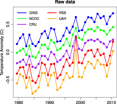
Figure 1. Five major global temperature records.
Download figure:
Standard imageTable 1. Warming rates in °C/decade, and lag in months, for each of the five temperature records and each of the three exogenous factors. Numbers in parentheses are standard errors in the final digits of the estimated values.
| Warming (°C/decade) | Lag (months) | ||||
|---|---|---|---|---|---|
| Raw | Adjusted | MEI | AOD | TSI | |
| GISS | 0.167(25) | 0.171(16) | 4 | 7 | 1 |
| NCDC | 0.162(22) | 0.175(12) | 2 | 5 | 1 |
| HadCRU | 0.156(25) | 0.170(12) | 3 | 6 | 1 |
| RSS | 0.149(40) | 0.157(13) | 5 | 5 | 0 |
| UAH | 0.141(44) | 0.141(15) | 5 | 6 | 0 |
All five data sets give warming rates which are consistent with one another. The largest difference is between the GISS and UAH data, but the difference fails statistical significance testing. Even so, the two lowest rates are for LT temperature while the three highest are for surface temperature. This suggests the possibility that the LT is warming more slowly than the surface, although we reiterate that such a suggestion is not supported with statistical significance.
4. Warming rates of adjusted data
Using multiple regression to estimate the warming rate together with the impact of exogenous factors, we are able to improve the estimated warming rates, and adjust the temperature time series for variability factors. The adjusted warming rates are listed in the second column of table 1, together with the best-fit lags for each of the three factors.
When exogenous influences are accounted for, the standard errors in the warming rate estimates are greatly reduced. This is especially true for the LT data sets, because these factors affect those data more strongly than they affect surface temperature. The warming rates are now in even better agreement, and it remains the case that none of the differences are statistically significant.
We also duplicated the analysis for the northern and southern hemispheres separately. Their warming rates (together with the global estimates) are plotted in figure 2. For both hemispheres, as for the globe, all five data sets give comparable warming rates with no statistically significant differences. However, we confirm the well-known fact that the northern hemisphere is warming more rapidly than the southern.

Figure 2. Estimated warming rates. Black dots are for global temperature, red for the northern hemisphere, blue for the southern hemisphere. Error bars are 2-σ.
Download figure:
Standard imageThe multiple regression also yields estimates of the coefficients for each of the exogenous factors. The coefficients of MEI, AOD and TSI influence are shown in figure 3. For both MEI and AOD, there is no indication of hemispheric differences but a strong indication of much greater influence on LT temperature than on surface temperature.
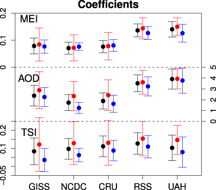
Figure 3. Coefficients of temperature response to MEI (multivariate el Niño index), AOD (aerosol optical depth) and TSI (total solar irradiance). Black dots are for global temperature, red for the northern hemisphere, blue for the southern hemisphere. We have plotted the negative of the AOD coefficient so that in all graphs, higher points represent stronger response.
Download figure:
Standard image5. Comparison of adjusted data sets
Figure 4 shows the adjusted data sets (with the influence of MEI, AOD and TSI, as well as the residual annual cycle removed) for monthly data. Two facts are evident. First, the agreement between the different data sets, even between surface and LT data, is excellent. Second, the global warming signal (which is still present in the adjusted data because the linear time trend is not removed) is far clearer and more consistent. When the fluctuations in temperature over the last 32 years (which tend to obscure the continuation of the global warming trend) are accounted for, it becomes obvious that there has not been any cessation, or even any slowing, of global warming over the last decade (or at any time during this time span). In other words, any deviations from an unchanging linear warming trend are explained by the influence of ENSO, volcanoes and solar variability.
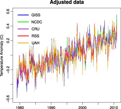
Figure 4. Adjusted data sets for all five sources, after removing the estimated influence of el Niño, volcanic eruptions and solar variations.
Download figure:
Standard imageThis is even clearer in the graph of annual averages of adjusted data in figure 5. It is worthy of note that for all five adjusted data sets, 2009 and 2010 are the two hottest years on record.

Figure 5. Annual averages of the adjusted data.
Download figure:
Standard imageTo look for changes in the warming rates over time, we computed the rate in adjusted data sets for different time intervals, for all start years from 1979 to 2005 and ending with the present. The results (figure 6) show no sign of a change in the warming rate during the period of common coverage. It is noteworthy that the noise reduction from removing the influence of exogenous factors enables warming to be established using shorter time spans than with raw data. All five data sets show statistically significant warming even for the time span from 2000 to the present.
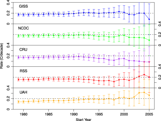
Figure 6. Trend rates from various starting years to December 2010, for all five adjusted data sets. Error bars are 2-σ.
Download figure:
Standard imageWe also tested for changes in the warming rate by fitting a quadratic function of time to the adjusted data sets. Only one of the data sets, the UAH series, showed a statistically significant quadratic term (p-value 0.03). It indicates acceleration of the warming trend at a rate of 0.006 °C/decade/yr. However, we regard this acceleration with skepticism because it shows in no other data set, not even the other satellite record.
5.1. Influence of ENSO, volcanoes and solar variation
We show the influence of the various factors on global temperature for a surface temperature record (GISS) and a satellite record (RSS) in figure 7, in order to illustrate the magnitude of their impact and to compare the results from surface- and a satellite-based data. ENSO has the largest overall impact, with a total range of variation of 0.39 °C for GISS and 0.64 °C for RSS. Volcanic aerosols have the second-largest influence, with range 0.35 °C for GISS and 0.52 °C for RSS. Solar variation, as characterized by TSI, shows the smallest total range of influence, 0.12 °C for GISS and 0.20 °C for RSS. Note that these ranges are for the temperature change induced by these factors, they are not coefficients of their influence, hence all are in units of degree celsius.
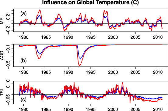
Figure 7. Influence of exogenous factors on global temperature for GISS (blue) and RSS data (red). (a) MEI; (b) AOD; (c) TSI.
Download figure:
Standard imageThe variances of the signal components corresponding to the influence of MEI, AOD and TSI are listed in table 2. This confirms that the influence of ENSO is greater than that of volcanic forcing and much greater than that of solar variation, and that both ENSO and volcanic forcing affect LT temperatures much more strongly than surface temperature. Also listed are the total variances of the raw data sets, and the variance of the residuals as well as R2 values (which gives the fraction of variance explained by the model) both for a simple linear trend with no other factors, and for the full model. The simple linear model explains over half the variance in surface temperature data but less than 40% for LT data. The full model explains 70%–80% of the variance for all five data sets. Not only do the included factors improve the fit for all data sets substantially, for LT data they roughly double the R2 values over those of a simple linear model.
Table 2. Variance attributable to MEI, AOD and TSI in the regression of global temperature for each of the five temperature records, as well as residual variances and the fraction of variance explained (R2 values) by two models. Total variance is for the raw data, that for individual factors is the variance of the temperature signal due to those factors, and residual variances and R2 values are for residuals from a linear fit to the raw data without additional factors, and from the full model (including all three factors and the linear trend).
| Total | MEI | AOD | TSI | Linear resid. | Full resid. | Linear R2 | Full R2 | |
|---|---|---|---|---|---|---|---|---|
| GISS | 0.0454 | 0.0053 | 0.0048 | 0.0008 | 0.0216 | 0.0139 | 0.525 | 0.693 |
| NCDC | 0.0368 | 0.0044 | 0.0026 | 0.0011 | 0.0143 | 0.0087 | 0.610 | 0.763 |
| CRU | 0.0341 | 0.0050 | 0.0031 | 0.0014 | 0.0134 | 0.0070 | 0.608 | 0.794 |
| RSS | 0.0487 | 0.0156 | 0.0107 | 0.0019 | 0.0296 | 0.0135 | 0.391 | 0.722 |
| UAH | 0.0490 | 0.0166 | 0.0132 | 0.0012 | 0.0320 | 0.0145 | 0.348 | 0.704 |
An interesting result is the time lags found. For volcanic eruptions the resulting cooling lags by about half a year, whereas the warming associated with El Niño events lags the multivariate ENSO index by 2–5 months. For ENSO the largest lag is found in the lower troposphere, whereas for solar forcing the lag in the surface data is larger. This is consistent with ENSO forcing the climate system from below (via ocean heat release) while solar irradiance forces the system from the top. The lags found here are consistent with those from Lean and Rind (2008) for the longer period 1889–2006, namely 6 months for volcanoes, 4 months for ENSO and 1 month for solar variations.
Finally, we list the linear trend in the signals due to ENSO, volcanic forcing and solar variation in table 3. The magnitudes of these trend contributions are quite small compared to the overall trends. In fact the net trend due to these three factors is negative for all data sets except UAH, for which it is zero. Hence these factors have not contributed to an upward trend in temperature data, rather they have contributed a very slight downward trend. Except for UAH data, the trend which is attributable to global warming is therefore very slightly greater than that which is observed in the unadjusted data.
Table 3. Trends in °C/decade of the signal components due to MEI, AOD and TSI in the regression of global temperature, for each of the five temperature records.
| MEI | AOD | TSI | |
|---|---|---|---|
| GISS | − 0.014 | 0.025 | − 0.014 |
| NCDC | − 0.014 | 0.019 | − 0.017 |
| CRU | − 0.015 | 0.020 | − 0.019 |
| RSS | − 0.022 | 0.038 | − 0.023 |
| UAH | − 0.023 | 0.041 | − 0.018 |
6. Conclusions
This analysis confirms the strong influence of known factors on short-term variations in global temperature, including ENSO, volcanic aerosols and to a lesser degree solar variation. It also emphasizes that LT temperature is affected by these factors much more strongly than surface temperature.
Perhaps most important, it enables us to remove an estimate of their influence, thereby isolating the global warming signal. The resultant adjusted data show clearly, both visually and when subjected to statistical analysis, that the rate of global warming due to other factors (most likely these are exclusively anthropogenic) has been remarkably steady during the 32 years from 1979 through 2010. There is no indication of any slowdown or acceleration of global warming, beyond the variability induced by these known natural factors. Because the effects of volcanic eruptions and of ENSO are very short-term and that of solar variability very small (figure 7), none of these factors can be expected to exert a significant influence on the continuation of global warming over the coming decades. The close agreement between all five adjusted data sets suggests that it is meaningful to average them in order to produce a composite record of planetary warming. Annual averages of the result are shown in figure 8. This is the true global warming signal.
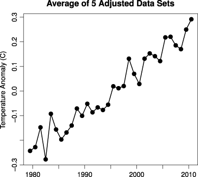
Figure 8. Average of all five adjusted data sets.
Download figure:
Standard imageIts unabated increase is powerful evidence that we can expect further temperature increase in the next few decades, emphasizing the urgency of confronting the human influence on climate.
Appendix.: Methods
Making best use of trend estimates requires also estimating the probable error associated with those values. This cannot be done treating the noise as white noise because the residuals from global temperature time series exhibit strong autocorrelation, which must be compensated for when estimating standard errors for the warming rates.
The most common method of compensating for autocorrelation in trend analysis is to treat the noise as a first-order autoregressive, or AR(1), process. In such a case the autocorrelation at a given lag j is

where ϕ is the autoregression coefficient. It is estimated by the lag-1 value of the sample autocorrelation function (ACF, usually according to the Yule–Walker estimate)  . Then one can compute a correction factor, which we can call the number of data per effective degree of freedom, as
Finally, the corrected standard error σc of an estimated trend rate c is the standard error σw one would estimate if the noise were white noise, multiplied by the square root of the number of data per effective degree of freedom

When the autocorrelation of the noise is positive (as is almost always the case), the corrected standard error σc is larger than the white-noise estimate σw, i.e., treating the noise as white noise underestimates the probable error in the trend rate.
Unfortunately, for global temperature time series such a procedure still underestimates the probable errors, because the noise is demonstrably different from AR(1) noise. This is illustrated in figure A.1, showing the estimated autocorrelation function of the residuals from a linear fit to GISS data from 1975 to the present. Clearly the AR(1) model (shown in red) underestimates the higher-order autocorrelations, so using that model will underestimate the probable error in the trend rate.
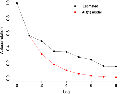
Figure A.1. Sample autocorrelation of residuals from a linear fit to raw GISS data, compared to the values for an AR(1) model.
Download figure:
Standard imageInstead, we adopt the more conservative model that the autocorrelation at lag j is still given by exponential decay with decay constant ϕ, but the lag-1 value is not necessarily equal to the exponential decay constant. Therefore the ACF is given by

This behavior corresponds to an ARMA(1, 1) process for the noise.
For a generic autocorrelation structure ordinary least squares regression still gives an unbiased estimate of the trend rate, but the correction factor for standard errors of the coefficients is (Lee and Lund 2004)

where ρj is the autocorrelation at lag j. When the noise is ARMA(1, 1), equation (A.5) becomes
and the correction to the standard error of the coefficients is still given by equation (A.3).
Hence for each data series, we used residuals from the models covering the satellite era to compute the Yule–Walker estimates  of the first two autocorrelations. Then we estimate the decay rate of autocorrelation as
Finally, inserting  and
and  into equation (A.6) enables us to estimate the actual standard error of the trend rates from the regression.
Footnotes
- 3
Available at http://data.giss.nasa.gov/gistemp/.
- 4
Available at www.ncdc.noaa.gov/cmb-faq/anomalies.html.
- 5
Available at www.cru.uea.ac.uk/cru/data/temperature/#datdow.
- 6
Available at www.remss.com/msu/msu_data_description.html#zonal_anomalies.
- 7
Available at http://vortex.nsstc.uah.edu/public/msu/t2lt/uahncdc.lt.
- 8
Available at www.esrl.noaa.gov/psd/people/klaus.wolter/MEI/table.html.
- 9
Available at http://data.giss.nasa.gov/modelforce/strataer/.