

Abstract
Record low snowpack conditions were observed at Snow Telemetry stations in the Cascades Mountains, USA during the winters of 2014 and 2015. We tested the hypothesis that these winters are analogs for the temperature sensitivity of Cascades snowpacks. In the Oregon Cascades, the 2014 and 2015 winter air temperature anomalies were approximately +2 °C and +4 °C above the climatological mean. We used a spatially distributed snowpack energy balance model to simulate the sensitivity of multiple snowpack metrics to a +2 °C and +4 °C warming and compared our modeled sensitivities to observed values during 2014 and 2015. We found that for each +1 °C warming, modeled basin-mean peak snow water equivalent (SWE) declined by 22%–30%, the date of peak SWE (DPS) advanced by 13 days, the duration of snow cover (DSC) shortened by 31–34 days, and the snow disappearance date (SDD) advanced by 22–25 days. Our hypothesis was not borne out by the observations except in the case of peak SWE; other snow metrics did not resemble predicted values based on modeled sensitivities and thus are not effective analogs of future temperature sensitivities. Rather than just temperature, it appears that the magnitude and phasing of winter precipitation events, such as large, late spring snowfall, controlled the DPS, SDD, and DSC.
Export citation and abstract BibTeX RIS

Original content from this work may be used under the terms of the Creative Commons Attribution 3.0 licence. Any further distribution of this work must maintain attribution to the author(s) and the title of the work, journal citation and DOI.
Corrections were made to this article on 31 August 2016. The acknowledgment of funding was updated.
1. Introduction
In 2015 the state of Oregon experienced widespread drought following the lowest winter snowpack since automated record keeping began in 1981 (NRCS 2015). At the end of water year 2015 (1 October 2014–30 September 2015), the United States Drought Monitor estimated that 67% of the state was in 'Extreme' (D3) drought conditions, resulting in a drought emergency declaration by the governor of Oregon and the release of $2.5 million in disaster relief (NRCS 2015). These conditions developed despite winter precipitation during 2014 and 2015 that mostly tracked the previous 30 year mean, in contrast to record low precipitation that characterized drought conditions in California (Diffenbaugh et al 2015, Mao et al 2015, Shukla et al 2015). 1 April snow water equivalent (SWE), on the other hand, was 68% and 11% of normal in 2014 and 2015, respectively. These represent the 8th and 1st lowest 1 April SWE in Oregon Snow Telemetry (SNOTEL) history, 1 April being the date on which SWE is normally maximum at most SNOTEL locations (Serreze et al 1999) and on which west-wide streamflow forecasts are largely based (McCabe and Dettinger 2002). These unique conditions have prompted many to speculate they may provide a harbinger of future conditions in a warming world, and an opportunity for managers to envision plans for the future (Thompson 2015, Walton 2015, Floyd 2016).
Speculation aside, these 35 year record low snowpack conditions are set against a backdrop of long-term climate warming, declining SWE, and associated shifts in streamflow throughout the American West (Hamlet et al 2005, Mote et al 2005, Fritze et al 2011, Safeeq et al 2013, Knowles 2015). These trends are strongly correlated with temperature, are not explained by natural variability (Hamlet et al 2005, Mote 2006, Abatzoglou 2011), and appear to be largely explained by decreased spring accumulation and/or increased spring melt, even at locations where winter accumulation has increased (Kapnick and Hall 2011). At broad scales they are at least in part attributed to anthropogenic warming (Barnett et al 2008, Pierce et al 2008, Hidalgo et al 2009). Given this attribution and current climate trajectories (Kirtman et al 2013), continued shifts toward less snow, more rain, and earlier snowmelt are considered likely. Looking toward such a future, the temperature sensitivity of Cascades snowpacks is of considerable interest (Casola et al 2009, Minder 2010, Luce et al 2014) and we ask the question: do these years serve as climate analogs for the sensitivity of mountain snowpacks in the maritime climate of the PNW?
This background and research question motivates our hypothesis that the 2014 and 2015 snow drought is an analog for the temperature sensitivity of SWE in the PNW. A simple way to test this hypothesis is to first establish the expected temperature sensitivity, and then compare with observations. Therefore, the first part of this paper describes a modeling experiment that estimates the temperature sensitivity of SWE for two watersheds (windward and leeward) in the Oregon Cascades, expressed in terms of changes in the magnitude and timing of SWE. The second part of this paper compares the modeled sensitivity of three key metrics—the peak SWE, the date of peak SWE (DPS), and the snow disappearance date (SDD)—to observed sensitivity derived from measurements of SWE at SNOTEL sites within the study watersheds and across the state of Oregon during the recent snow drought. These snow metrics are relevant to different stakeholders and we aim to demonstrate for which metrics the recent snow drought may serve as an analog for the temperature sensitivity of SWE in the study region.
2. Study region
The Cascades mountain range extends from southern British Columbia to northern California (figure 1). Our study focuses on two watersheds in the central Oregon Cascades: the west side (windward) McKenzie River Basin (MRB, 3040 km2) and east side (leeward) Upper Deschutes River Basin (UDRB, 870 km2). Snow provides a critical natural reservoir for hydropower, irrigated agriculture, municipalities, and federally protected native cold-water fish in the region, as is common throughout the western US. The Natural Resources Conservation Service (NRCS) measures temperature, precipitation, and SWE at five SNOTEL sites and SWE at two snow courses (snow measurement transects) in the study watersheds, which are part of a larger US-wide snow monitoring network that facilitates water resources management in snow dependent regions.
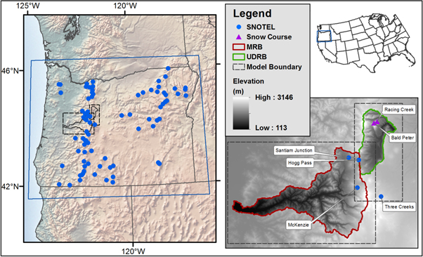
Figure 1. Map of the study region showing the location of the McKenzie River Basin (122°24'10'' W, 44°12'9'' N) and Upper Deschutes River Basin (121°39'35'' W, 44°32'35'' N) watershed boundaries, modeling domain boundaries, SNOTEL and Snow Course monitoring stations (http://wcc.nrcs.usda.gov/snow/), and elevation in the region.
Download figure:
Standard image High-resolution imageElevations in the watersheds range from 400 to 3200 m. Above 1800 m the topography is characteristic of a volcanic plateau segmented by large volcanic peaks; from 400 to 1800 m the watersheds are characterized by steep and highly dissected terrain, typical of the Pacific Arc maritime mountain ranges (Tague and Grant 2004, Jefferson et al 2010). According to the Parameter Regressions on Independent Slopes Model (PRISM) climatology, basin wide mean annual precipitation ranges from 2200 to 1200 mm and mean annual air temperature from 8.3 °C to 6.8 °C, for the MRB and UDRB, respectively (Daly et al 2008).
3. Data and methods
3.1. SnowModel setup, input data, and evaluation
We developed a 23 year climatology of SWE in the study watersheds for the period 1989–2011 using SnowModel, a spatially-distributed snow accumulation and energy balance ablation model (Liston and Elder 2006a, 2006b). We ran the model at 100 m horizontal grid spacing with a daily time step. To represent the distinct windward and leeward climates of the study watersheds, we defined separate modeling domains (figure 1) and defined unique temperature lapse rates for the MRB and UDRB. Lapse rates were computed from 30 arcsecond (800 m) PRISM monthly timeseries of minimum and maximum air temperature using standard least-squares linear regression, which were then interpolated between months and averaged to create daily lapse rates for each watershed. Precipitation (PPT) was partitioned into snowfall (SF) versus rainfall with a linear function of air temperature:
where TS (−0.5 °C) is the temperature below which all precipitation is defined to be snowfall and TR (1.75 °C) is the temperature above which all precipitation is defined to be rainfall. The United States Army Corps of Engineers developed equation (1) from measurements of snowfall in the PNW (USACE 1956). We acknowledge the limitations of this empirical approach (Dai 2008, Marks et al 2013, Safeeq et al 2016) and provide a discussion of the uncertainty and how we handled it in the supplementary material.
Model inputs include (1) spatially distributed fields of precipitation, air temperature, wind speed, wind direction, and relative humidity; and (2) spatially distributed fields of topography and vegetation type. We used daily average air temperature, daily total precipitation, and daily average relative humidity gridded at 1/16° (5 × 7 km) (Livneh et al 2013), and the National Center for Environmental Prediction-National Center for Atmospheric Research (NCEP–NCAR) daily average wind speed and direction gridded at 2.5° spatial resolution (Kalnay et al 1996). Air temperature and precipitation were bias corrected with the PRISM 800 m monthly time series using the delta and ratio methods, respectively (Watanabe et al 2012). Wind and humidity data were bilinearly interpolated to the PRISM 800 m grid. The 800 m grids were used as the final model inputs, which were interpolated to the 100 m topography during model setup using SnowModel's built-in MicroMet utility. Topography and vegetation were resampled to 100 m resolution from the United States Department of Interior 30 m National Elevation Dataset digital elevation model and the 2011 National Land Cover Database land cover definitions (Gesch et al 2002, Fry et al 2011).
We used daily data from four automated SNOTEL stations ('test' sites) in the study region to evaluate SnowModel. The test sites span the windward and leeward sides of the study region and range in elevation from 1143 to 1733 m (figure 1). Some limited model development and calibration was required to achieve adequate model performance. This included adding a parameterization for retention and drainage of liquid water in the snowpack and a Monte Carlo parameter calibration routine (supplementary material).
3.2. Temperature sensitivity model experiment
Following Casola et al (2009), the effect of a change in surface air temperature on snow accumulation and melt can be assessed with a 'temperature sensitivity' parameter:

where  is a snow-related metric,
  is a change in surface air temperature, and

is the temperature sensitivity of  The first term on the rhs of (3) is the 'direct' temperature sensitivity and represents changes in
  that result directly from changes in air temperature. The second term on the rhs of (3) represents indirect changes in
  due to a variable that is dependent on
  for example an increase in local precipitation due to an increase in specific humidity with air temperature. In this study, we ignore all indirect effects and focus solely on the 'direct' temperature sensitivity,
  which we term
  This choice simplifies the analysis for reasons of tractability, but also introduces uncertainty by ignoring potential indirect effects (e.g. Minder 2010). Following on this, if an estimate of
  is known, equation (2) can be used to predict
  For simplicity we adopt the notation:

where  is a change in
  that results from a change in air temperature,
  as predicted by an estimate of
  In this study, we use a number of metrics for
  described below.
We modeled  using the 'delta' method (Hay et al 2000), where the historical daily air temperature data were uniformly increased by +2 °C (T2) and +4 °C (T4) and precipitation increased by +10% (P10). The temperature increases represent the expected mid- to late 21st century average changes for the Pacific Northwest (PNW) region from 20 global climate models and two greenhouse gas emissions scenarios (B1 and A1B) (Mote and Salathé 2010). For precipitation, the magnitude and direction of projected 21st century change for the PNW is highly uncertain (Safeeq et al 2016). Thus, a simple 10% precipitation increase was chosen to explore the effect of increased P on
  The perturbed forcing data were used as input to the model to develop time series of SWE for each scenario, referred to as T2, T4, T2P10, and T4P10.
For each scenario we computed the mean per-pixel change in SWE (dSWE, m) and cumulative snowfall (dSF, m) on each calendar day, the mean per-pixel change in the date of peak SWE (dDPS, days), the snow disappearance date (dSDD, days), and duration of snow cover (dDSC, days), and the change in basin snow-covered area (dSCA, m2) on the date of peak basin volumetric SWE, relative to the reference period. These quantities were in turn used to calculate basin-scale area-weighted estimates of S for SWE, SF, and SCA on the basin DPS and 1st April, normalized by their reference period value and expressed as percent change (% °C−1). For the timing metrics (DPS, SDD, SCD), we express estimates of S as absolute change e.g. dSDD/dT (days °C−1).
To compare model findings with statewide SWE patterns during 2014 and 2015, we predicted statewide SWE anomalies with equation (4), using a model-derived empirical relationship between air temperature and S. We selected the metrics peak SWE, DPS, and SDD for this analysis. To achieve this, we binned grid cells by their mean DJFM (defined here as the snow accumulation season) air temperature, and computed the mean value of S for each 0.1 °C bin. We used these values as look-up tables that defined S as empirical functions of mean DJFM air temperature for each metric. We then computed the 2014 and 2015 PRISM DJFM air temperature anomalies to approximate  and solved equation (4) for
 and
and  for PRISM grid cells with mean DJFM air temperature <4 °C and total DJFM precipitation >15 cm (values that bound the range of maximum DJFM air temperature and minimum 1 April cumulative precipitation computed from the SNOTEL data):


where  is the look-up table sensitivity for each metric and
  is the PRISM DJFM air temperature anomaly. To evaluate the robustness of the extrapolation, predicted
  was compared to observed 2014/2015 peak SWE, DPS, and SDD anomalies
  for each SNOTEL station in the state of Oregon with a period of record beginning 1981 or earlier.
Previous studies have used empirical methods e.g. linear regression between interannual variations in air temperature and SWE ('temporal analogs'; Mote 2006, Stoelinga et al 2010, Luce et al 2014), physically-based model simulations (Sproles et al 2013), or a combination of the two approaches (Mote et al 2005, Casola et al 2009) to estimate SWE temperature sensitivity in the PNW region. Luce et al (2014) presented a third method, termed 'spatial analogs' that used nonlinear polynomial regression between spatial variations in air temperature and SWE. These studies have led to some disagreement (Mote et al 2008, Casola et al 2009, Luce et al 2014), thus it is important to note that our approach is both similar (e.g. the physical model) and unique (e.g. the extrapolation procedure) from these previous methods. We discuss similarities and distinctions between ours and previous findings in section 5. Luce et al (2014) provide a detailed discussion of previous work on the topic.
4. Results
4.1. Modeling and diagnosing sensitivity of SWE metrics in the study watersheds
Basin-wide modeled declines in peak SWE and the concurrent loss of SCA for the four scenarios are shown in figure 2. Peak basin-mean SWE decreased by 59% and 88%, and SCA on the basin DPS decreased by 40% and 69%, for the T2 and T4 scenarios, respectively. The 10% increase in precipitation had a relatively small effect on decreases in SWE and SCA, but the effect was elevation (and thus temperature-regime) dependent (figure 3). In our relatively warm basins, the basin-mean SWE losses were nominally offset by 7% and 2%, and SCA losses by 1% and 1%, for the T2P10 and T4P10 scenarios, respectively. Expressed as basin-mean sensitivities, 

 and
and  Shifts in timing metrics (DPS, SDD, DSC) were also large and insensitive to increased precipitation (table 1).

Figure 2. Maps of mean peak SWE and SCA for the MRB and UDRB for the reference period, and for the T2, T4, T2P10, and T4P10 scenarios. Locations of SNOTEL stations and snow course transects within the watersheds used in this study are shown as blue circles and purple triangles, respectively. Monthly measurements of SWE at snow course transects provide a key source of information used by the NRCS to develop summertime streamflow forecasts (http://wcc.nrcs.usda.gov/factpub/wsf_primer.html).
Download figure:
Standard image High-resolution image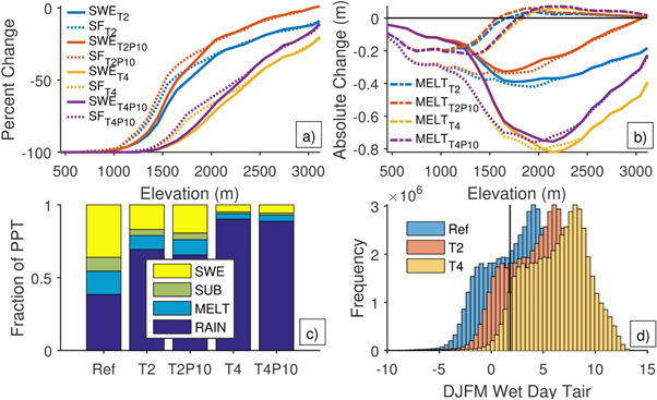
Figure 3. The mean (a) percent change in cumulative SWE and SF on the DPS, averaged over 100 m elevation bands (b) absolute change in SWE, SF, and cumulative snowmelt on the DPS, averaged over 100 m elevation bands; (c) the partitioning of precipitation into rainfall, SWE, snowmelt, and sublimation (canopy + surface), cumulative on the DPS; and (d) the distribution of mean modeled air temperature on modeled wet days in the study watersheds for the reference period and for the T2 and T4 scenarios. The rain–snow partitioning temperature (1.75 °C) used in this study is shown as a vertical black line. With incremental warming, significant fractions of snowfall events shift to rainfall events, but the area shifted diminishes with increased warming.
Download figure:
Standard image High-resolution imageTable 1. The basin-mean sensitivity of each metric for each scenario, and the mean modeled sensitivity at basin test sites compared to observed sensitivities for 2014 and 2015. Snowfall is not measured at the test sites and snow-covered area is not a point-scale metric.
| Basin-mean | Test-sites | |||||||
|---|---|---|---|---|---|---|---|---|

|

|

|

|

|

|

|

|
|
| Peak SWE (%) | −29 | −26 | −22 | −22 | −26 | −33 | −21 | −22 |
| 1 April SWE (%) | −31 | −27 | −23 | −22 | −28 | −35 | −23 | −25 |
| Peak SF (%) | −28 | −25 | −21 | −21 | — | — | — | — |
| 1 April SF (%) | −26 | −24 | −21 | −20 | — | — | — | — |
| Peak SCA (%) | −20 | −19 | −17 | −17 | — | — | — | — |
| 1 April SCA (%) | −25 | −23 | −21 | −20 | — | — | — | — |
| DPS (days) | −13 | −13 | −13 | −13 | −11 | 2 | −11 | −19 |
| DSC (days) | −34 | −31 | −31 | −29 | −28 | −32 | −24 | −21 |
| SDD (days) | −25 | −23 | −23 | −22 | −21 | −32 | −19 | −22 |
These modeled changes in SWE were primarily controlled by shifts from snowfall to rainfall, both on a basin-scale (table 1), and across the entire elevation range (figures 3(a) and (b)). The largest relative decreases in SWE (figure 3(a)) occurred at low elevations where absolute decreases (figure 3(b)) were small. The largest absolute decreases occurred at elevations between 1700 and 2500 m where the majority of SWE accumulated during the reference period. Changes in cumulative snowmelt (figure 3(b)) appeared to be a consequence of the reduced SWE as opposed to a cause, as total snowmelt decreased at elevations up to 1700 m. Above 1700 m, snowmelt increased slightly, but increased melt was small relative to the reduction in snowfall. The strong dependence of these changes on modeled shifts from snowfall to rainfall is demonstrated by the basin-scale mean wet-day air temperature distribution (figure 3(d)). The nonlinearity of modeled  suggested by comparing basin-scale
  to
to  is at least in part explained by the step-function shift toward warmer temperatures we apply to this distribution, however the true effect will depend on changes to the statistical moments of this distribution in both space and time under future climate.
4.2. Comparing the T2 and T4 sensitivities to observations from 2014 and 2015 at SNOTEL test sites
During 2014 and 2015, the mean DJFM air temperature anomalies at the four SNOTEL test sites were +1.3 °C and +3.9 °C, respectively. Basin-averaged PRISM air temperature anomalies were +1.0 °C and +3.5 °C, respectively. Cumulative SNOTEL precipitation for 2014 and 2015 on 1 April was 103% and 92% of normal, whereas basin-averaged PRISM precipitation was 97% and 90% of normal, respectively. These unique meteorological conditions roughly mirror what is expected for the region by mid- to late 21st century (Mote and Salathé 2010) and thus motivate our comparison between the modeled T2/T4 SWE, measured SWE during 2014/2015, and corresponding sensitivities (figure 4).

Figure 4. The 30 year mean measured precipitation and SWE compared to (a) WY 2014 conditions and the T2 scenario averaged across the four test sites and (b) WY 2015 and the T4 scenario averaged across the four test sites. (c) and (d) Same but for air temperature. The SNOTEL DJFM precipitation and air temperature anomalies are noted in blue and red text, respectively.
Download figure:
Standard image High-resolution imageDuring 2014, the peak SWE anomaly was −40%, DPS was 3 days later than normal (1 April), and SDD was 39 days earlier than normal (3 June). The T2 peak SWE anomaly was −53%, DPS was 24 days earlier (9 March), and SDD was 41 days earlier (1 June). During 2015, the peak SWE anomaly was −83%, DPS was 73 days earlier than normal (16 January), and SDD was 82 days earlier than normal (21 April). The T4 peak SWE anomaly was −85%, DPS was 39 days earlier (23 February), and SDD was 80 days earlier (23 April). Expressed as sensitivities,  (−22%) was strikingly similar to our estimate for
  (−21%), but
  was underestimated by
  The timing metrics
 and
and  showed varying levels of agreement between modeled and observed sensitivity but the modeled
  was notably inconsistent with observations during both years (table 1).
Further examination of figure 4 shows that temporal SWE variability during 2014 and 2015 corresponded to the sub-seasonal phasing of precipitation and temperature anomalies (which the mean modeled sensitivities necessarily smooth out), shedding light on the deviation between observed and modeled 
 and
and  This behavior was consistent across sites during 2014, when early winter SWE was below average but peaked 3 days later than normal on 1 April, and during 2015 when the opposite phasing occurred, SWE peaked 73 days early on 16 January, and melted out 82 days early on 21 April, as opposed to more modest shifts predicted by
  and
and  (table 1). The effect of storm phasing was particularly strong in 2014 when a very cold and wet February boosted record low January snowpacks and the resulting 1 April SWE was recorded as the 8th lowest in the 35 year period of record. Each site showed a pattern of recovery that resulted in a normal DPS. Contrasting behavior was observed during 2015 when early season precipitation coincided with anomalously warm temperature and the basin-wide temperature anomaly remained above 3.4 °C from January through March, with no recovery as in 2014. As a result, SWE peaked on 16 January and the lowest 1 April SWE in 35 years was recorded despite 90%-of-normal 1 April precipitation.
4.3. Extrapolating basin-derived modeled sensitivities statewide
These results demonstrate that 2014/2015 peak SWE in our study watersheds closely resembled the T2/T4 peak SWE, but also that observed and modeled DPS and SDD were less consistent in both absolute terms and when expressed as S. Here, we show how the basin-derived S predict observed D across a broader geographic area during 2014 and 2015. We first note that figure 3 suggests  strongly depends on elevation, a result noted by many (Knowles and Cayan 2004, Mote 2006, Tennant et al 2015). However, this dependence is largely due to the dependence of air temperature on elevation (Mote 2006). Thus, a more general approach is to define
  as a function of mean air temperature during the snow accumulation season. We use these relationships (figure 5), as opposed to the basin-mean sensitivities, to extrapolate our estimates of
  across the state (figure S2), and to test the degree to which observed conditions during 2014 and 2015 correspond to those predicted by the modeled sensitivities.

Figure 5. The model-derived empirical relationships (look-up tables) between mean DJFM air temperature and (a) peak SWE sensitivity  (b) the snow-disappearance date sensitivity
  (c) the date of peak SWE sensitivity
  and (d) the duration of snow cover sensitivity
  for the T2 and T4 scenarios. The
  sensitivities 'saturate' at 50% and 25% for the T2 and T4 scenarios, respectively, indicating that pixels above the corresponding ordinate temperature become snow-free (100% loss). The
 and
and  truncate at these same temperatures as there is no snow to compute a change (only the T4 curve saturates within the range of temperatures in the study region).
Download figure:
Standard image High-resolution imageStatewide,  predicted by
  corresponded reasonably well to observed anomalies during 2015 (r2 = 0.52; figure 6(d)) when winter conditions were unusually warm (+3.3 °C at >1000 m) and precipitation relatively normal (−1% at >1000 m), with minimal spatial variability throughout the state (figure S3). During 2014, precipitation variability (−17% at >1000 m) likely contributed to the underpredicted peak SWE anomalies (r2 = 0.39; figure 6(a)). In general, there was much more variability in the observed response to conditions in 2014 and 2015 than the mean sensitivity functions predicted (figure 6). Only peak SWE showed similar spread across the observations as the extrapolated predictions. The timing metrics DPS and SDD were particularly scattered. These results are consistent with the plot scale analysis where the phasing of precipitation appeared to determine the temporal character of SWE, which likely differed from phasing across the state. Further, the 1σ spread in the sensitivity functions (figure 5) suggest substantial uncertainty across relatively narrow climatic bands, especially at warmer locations and for greater magnitudes of warming.

Figure 6. The predicted peak SWE, DPS, and SDD anomalies  compared to observed anomalies
  at each of the 69 SNOTEL stations shown in figure 1. The best fit line and mean
  versus mean
  are plotted as dashed line and yellow squares, respectively.
Download figure:
Standard image High-resolution image
When averaged across all sites, the 2014 statewide mean peak SWE anomaly was −36%, DPS was 9 days earlier than normal on 13 March, and SDD was 52 days earlier than normal on 19 April. Mean values predicted by  were −30%, 17 days, and 27 days (for comparison see yellow squares, figure 6). The 2015 mean peak SWE anomaly was −67%, DPS was 56 days earlier than normal on 26 January, and SDD was 101 days earlier than normal on 1 March. Mean values predicted by
  were −68%, 40 days, and 64 days. The cool temperatures and late precipitation during spring 2014 resulted in a DPS later than predicted, but the SDD occurred 25 days earlier than predicted. The early precipitation and warmth during winter 2015 resulted in a DPS 26 days earlier than predicted, and the SDD 37 days earlier than predicted. Expressed as sensitivities for the Oregon SNOTEL network,
  = 29% °C−1,
  = 30% °C−1,
  = 20% °C−1, and
  = 20% °C−1.
5. Discussion
While a +4 °C warming may seem extreme in the near future, it is well within the bounds of the 1.3 °C–5.1 °C warming projected by mid- to late 21st century for the PNW (Dalton et al 2013). The warm winters of 2014 and 2015 in Oregon may provide a cautionary glimpse of winter temperature conditions in this maritime region, but our results suggest these winters are not ideal analogs for all metrics of the direct SWE temperature sensitivity presented here.
Peak SWE sensitivities were similar to the 22–30% °C−1 reported in previous physically-based modeling studies of basin-scale 1 April SWE sensitivity in this region (Casola et al 2009, Sproles et al 2013), and showed some predictive ability especially when aggregated to mean values. However, empirical findings suggest temperature sensitivity is nonlinear both with elevation (temperature regime) and degree of warming (Luce et al 2014). Thus, the SWE sensitivity of individual watersheds will depend on both the hypsometric distribution of air temperature (Tennant et al 2015) and the degree of regional warming, which may be amplified by elevation-dependent warming trends (Mountain Research Initiative EDW Working Group 2015). In the PNW, uncertainties for projected changes in precipitation may outweigh the temperature sensitivity of SWE. The reader is advised to consult figure 11 of Luce et al (2014) to contextualize the temperature-regime from which our results are derived.
Our study provides evidence that 2014 and 2015 are reasonable climate analogs for peak SWE sensitivity, but not necessarily for the DPS or SDD. Such findings provide insights into the spatial distribution and climatic causes of snowpack sensitivity, yet it remains difficult to relate model coefficients, response surfaces, and model output to conditions from individual years that are hypothesized to resemble warmer futures. While it may be attractive to use individual years to visualize a warmer future, care must be taken to understand the limits to such an approach. Peak SWE may work reasonably well as an analog metric because it integrates the effects of individual storms over the course of the winter whereas DPS and SDD can be strongly influenced by individual storm events and are not likely to represent any sort of future average conditions. At the same time, the common practice of presenting the potential impacts of climate change on water resources in terms of mean shifts in variables of interest (e.g. the sensitivities presented here) may not represent any sort of future actual conditions.
The ability to diagnose sensitivity based on changes to water balance partitioning for a specific elevation range or spatial scale is a key strength of spatially distributed models such as SnowModel that may be useful to guide management and research directions. For example, our results suggest that warming may lead to large decreases in mid-winter snowmelt, increased rainfall, and earlier snow disappearance, which may change the amount and timing of soil water available for evapotranspiration in forested basins such as the study region, with unknown consequences for forest productivity (Garcia and Tague 2015, Harpold 2016). From a management perspective, our results suggest that on average, 70% of 1 April SWE accumulates above the SNOTEL station network in the MRB, compared to 40% for the UDRB, due to higher elevation network coverage in the UDRB. With a 2 °C and 4 °C warming, the modeled snowline shifted upward such that 94% and 99% of 1 April SWE accumulated above the MRB network, compared to 57% and 90% for the UDRB. In either case, as climate warming proceeds, the vast majority of SWE will likely accumulate where there are no historical measurements, rendering the predictive capacity of our monitoring networks obsolete.
The results presented here are derived from a single hydrologic model employing a widely used, but relatively simple, temperature-based snowfall parameterization. The lapse rate-based temperature interpolation does not capture the effects of inversions and storm-scale lapse rate variability. Our climate scenarios ignore dynamical changes to the climate-snow system that are expected to result from warming (Mankin and Diffenbaugh 2014). These are important sources of uncertainty in our estimate of temperature sensitivity, and future work should focus on constraining this uncertainty. In particular, in addition to precipitation magnitude variability, there is a critical need to understand how storm phasing and associated freezing levels may respond to climate warming in order to anticipate changes to the timing of SWE accumulation and ablation.
The extrapolation procedure was based on temperature, ignoring other variables such as topography and vegetation that influence SWE through modification of surface mass and energy fluxes. The 1σ spread in figure 5 demonstrates large variability across relatively narrow climatic bands in our study watersheds. This uncertainty is underscored by the simplistic representation of forest cover used in this and most hydrologic model studies. We do not explicitly model the conditions of 2014 and 2015, nor do we use future climate scenarios, weather generators, or other ensemble-based techniques (e.g. Mankin et al 2015) to force the model and quantify our results in terms of statistical likelihoods. These results are not a critique of the sensitivity approach in a general sense, but instead highlight the limitations of the approach as well as the utility of extreme events for anticipating mean changes in snow metrics.
6. Conclusion
Is the recent snow drought an analog for winter warming sensitivity of Cascades snowpacks? In terms of peak SWE accumulation the snow drought was well approximated by the mean temperature sensitivity presented here. However, mean sensitivities may not be relevant at the seasonal scale for metrics such as the DPS, SDD, and DSC, and therefore may have less utility as planning tools. Future work should test the robustness of this finding over longer time periods as opposed to a single extreme event, and within the context of ensemble simulations and/or internally consistent future climate simulations. Nevertheless, in as far as our modeled sensitivity is representative of future mean conditions, we find that for each 1 °C of warming, there is a 28% shift from snowfall to rainfall, SWE decreases up to 30%, the DPS advances by up to two weeks, and the SDD advances by over three weeks; however, these basin-scale values are temperature-regime dependent. With a 2 °C warming, low- and mid-elevation snow is virtually eliminated. The implications of these findings will differ based on stakeholder needs, for example flood control and irrigation timing, hydropower generation, and snow dependent habitat, and highlight the critical role that elevation plays in controlling the sensitivity of water resources to warming in mountainous regions.
Acknowledgments
This research was funded by a USGS award through the Northwest Climate Science Center (G12AC20452) and an NSF Water Sustainability and Climate award (EAR-1039192). The first author thanks the College of Earth, Ocean, and Atmospheric Sciences and the Water Resources Graduate Program, Oregon State University for graduate student funding that supported the completion of this research. The authors thank Charlie Luce and two anonymous reviewers for their insightful and timely comments that significantly improved the quality of the manuscript.