

Abstract
Many studies have used thermal data from remote sensing to characterize how land use and surface properties modify the climate of cities. However, relatively few studies have examined the impact of elevated temperature on ecophysiological processes in urban areas. In this paper, we use time series of Landsat data to characterize and quantify how geographic variation in Boston's surface urban heat island (SUHI) affects the growing season of vegetation in and around the city, and explore how the quality and character of vegetation patches in Boston affect local heat island intensity. Results from this analysis show strong coupling between Boston's SUHI and vegetation phenology at the scale of both individual landscape units and for the region as a whole, with significant detectable signatures in both surface temperature and growing season length extending 15 km from Boston's urban core. On average, land surface temperatures were about 7 °C warmer and the growing season was 18–22 days longer in Boston relative to adjacent rural areas. Within Boston's urban core, patterns of temperature and timing of phenology in areas with higher vegetation amounts (e.g., parks) were similar to those in adjacent rural areas, suggesting that vegetation patches provide an important ecosystem service that offsets the urban heat island at local scales. Local relationships between phenology and temperature were affected by the intensity of urban land use surrounding vegetation patches and possibly by the presence of exotic tree species that are common in urban areas. Results from this analysis show how species composition, land cover configuration, and vegetation patch sizes jointly influence the nature and magnitude of coupling between vegetation phenology and SUHIs, and demonstrate that urban vegetation provides a significant ecosystem service in cities by decreasing the local intensity of SUHIs.
Export citation and abstract BibTeX RIS
1. Introduction
Urban areas occupy a small proportion of the global land surface, but have a large impact on local-to-global environmental systems. At local scales, urban land use modifies the physical and geometric properties of land surfaces relative to natural land cover, which alters surface energy and radiation budgets (Arnfield 2003). In particular, the presence of buildings, roads, and other impervious surfaces increases absorption of shortwave radiation, decreases energy loss via emission of longwave radiation, and reduces evapotranspiration relative to adjacent natural land cover (Oke 1976, Landsberg 1981). As a result, near-surface air temperatures tend to be 0.5 °C–3.0 °C higher than surrounding rural areas (Bounoua et al 2015, Jochner et al 2015 and citations therein)—a phenomenon known as the urban heat island (UHI). Within cities, however, trees and other types of vegetation provide significant local cooling via shading and leaf transpiration, and supply additional ecosystem services through carbon sequestration and provision of habitats for flora and fauna (Nowak and Crane 2002, Wilby and Perry 2006, Peters et al 2010, Briber et al 2013).
Vegetation phenology—the annual cycle of leaf emergence, development, and senescence of leaves (and flowers)—is strongly controlled by temperature in many ecosystems, and is therefore a widely-used diagnostic of climate change impacts on natural ecosystems (Chmielewski and Rötzer 2001, Parmesan and Yohe 2003). In biomes where temperature is the dominant control on phenology, UHIs have the potential to alter the growing season of vegetation in cities. Indeed, recent studies have demonstrated that UHI's can lead to earlier emergence of leaves and flowers in spring or delayed senescence in fall. For example, Jochner et al (2012) used 30 years of ground observations to show that urbanization in three German cities advanced the timing of spring phenophases for nine deciduous species by 2.6–7.6 days between 1980 and 2009. In an earlier study, Rötzer et al (2000) found 1.5–4.0 day advances in the timing of urban spring flowering relative to surrounding rural areas for four species in ten European cities.
While these results provide compelling evidence of the impact of UHIs on vegetation phenology, studies based solely on ground observations provide limited information regarding the spatial complexity of phenology in urban areas. Further, comparison of results across ground-based studies is challenging because different studies use different species, methods of analysis, and data collection protocols (Denny et al 2014, Gill et al 2015). Satellite remote sensing, on the other hand, provides an objective and quantitative means for assessing patterns in land surface phenology—i.e., spatially integrated measurements of seasonal variation in surface properties measured from remote sensing—that can be examined at local-to-global scales (de Beurs and Henebry 2004). Specifically, time series of vegetation indices such as the normalized difference vegetation index (NDVI) and the enhanced vegetation index (EVI) derived from coarse spatial resolution sensors such as AVHRR (1–8 km), SPOT-VEGETATION (1 km) and MODIS (250–500 m) have been widely used to estimate phenological metrics that measure the timing of spring and autumn phenology (Moulin et al 1997, White et al 2002, Zhang et al 2003, Ahl et al 2006, Delbart et al 2006, Walker et al 2015). While observations from AVHRR, MODIS, and SPOT provide high frequency observations over large areas, the relatively coarse spatial resolution of these instruments presents substantial challenges for studies focused on urban areas, which are highly heterogeneous relative to the spatial resolution of these sensors (Jat et al 2008). Further, exotic and ornamental species, which are common in cities and often exhibit phenological behavior that is different from that of native species, can affect the observed signature of climate on plant phenology (Jim and Liu 2001, Körner and Basler 2010).
Within this general framework, the goals of this paper are to exploit new remote sensing-based capabilities to quantify and characterize how UHI intensity affects vegetation phenology in the Boston metropolitan area at landscape-scale, and to improve understanding of how spatial variation in land use and land cover control both the intensity of Boston's UHI and its impact on phenology. To do this, we used estimates of phenophase transition dates from a newly developed method that uses 30 m Landsat data, Landsat-derived land surface temperature (LST) data and maps of impervious surface area (ISA) and tree canopy cover to address three questions: (1) How does the UHI influence spring and autumn phenology across Boston's urban-rural gradient? (2) How does phenology vary within the city of Boston and how much of this spatial variation is explained by local variation in land cover and land use? And, (3) does the nature of land use surrounding vegetation patches affect UHI intensity at local scales? Note that because we use LSTs derived from remote sensing and not air temperatures to measure the intensity of Boston's UHI, hereafter, we refer to this as the surface urban heat island (SUHI).
2. Methods
2.1. Study region
Our study region includes the Greater Boston metropolitan area (figure 1), encompassing ∼12 000 km2 of residential and commercial land use in and around Boston, with surrounding rural areas composed of northern hardwood and oak/hickory forests inland and woody wetlands along the coast. Elevation in the study region ranges from 0 to 192 m above sea level and the climate is classified as humid continental. Precipitation is uniform throughout the year, but temperatures are highly seasonal with relatively warm summers and cold winters. In response, deciduous vegetation in the region has well-defined phenology that is primarily controlled by temperature (e.g., Richardson et al 2006, Friedl et al 2014).
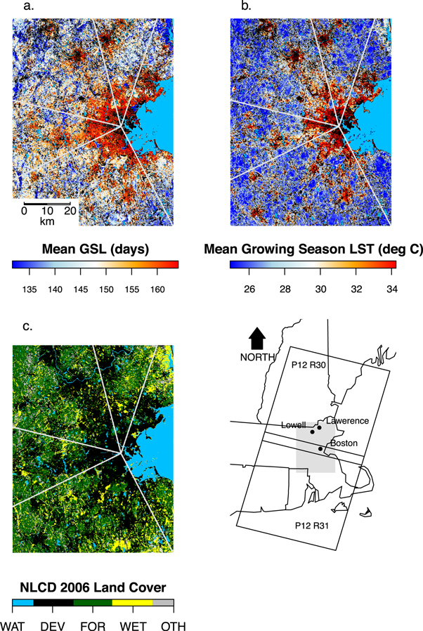
Figure 1. (a) Long-term mean growing season length (GSL), (b) long-term mean growing season land surface temperature (LST) and (c) land cover (WAT = water; DEV = developed; FOR = forest; WET = wetlands; OTH = other) maps of the study region. In panels (a) and (b), blue corresponds to water and black corresponds to pixels where the correlation between observed and spline-predicted EVI is less than 0.85. The black boxes in the lower right hand panel are the Landsat TM/ETM+ scenes with corresponding path (P) and row (R) numbers labeled.
Download figure:
Standard image High-resolution image2.2. Landsat-based phenology detection
We used all available Landsat TM and ETM+ images from the United States Geological Survey with less than 90% cloud cover for two scenes that cover the Greater Boston metropolitan area (Path 12, Rows 30 and 31; see figure 1). Image digital numbers were converted to surface reflectance using the Landsat Ecosystem Disturbance Adaptive Processing System algorithm (Masek et al 2006), and observations contaminated by clouds, cloud shadows, and snow and ice were identified and removed using the Fmask algorithm (Zhu and Woodcock 2012). The final data set included a total of 1175 TM and ETM+ images spanning the period from 1984 to 2013.
To map information related to green leaf phenology, we used the Landsat Phenology Algorithm (LPA; Melaas et al 2013) to estimate the long-term average and annual day of year associated with leaf emergence (start of spring; SOS) and autumn senescence (end of season; EOS) at 30 m spatial resolution. Because the LPA was originally designed for application over forested areas with relatively dense tree cover (i.e., with relatively high maximum summertime EVI), we incorporated two modifications to support detection of phenology in areas with lower tree cover (i.e., urban areas). First, instead of estimating separate spring and autumn logistic curves to model seasonal variation in Landsat EVI, we used smoothing splines to model the mean annual phenology at each location, and then normalized the resulting function at each pixel to vary between 0 and 1. Similar to Melaas et al (2013), the long-term average SOS and EOS at each pixel were estimated based on the date when the normalized spline reached 50% of the spring and autumn amplitude, respectively. Second, using a high-resolution canopy cover map of Boston (see below), we found that arbitrarily defined ranges for long-term mean winter background and peak summer EVI significantly underestimates deciduous tree coverage within the city. Alternatively, since trees are less moisture-limited than grasses and shrubs, they exhibit less interannual variability in summer EVI and, hence, greater agreement (i.e., higher correlation) with a long-term mean fitted cubic spline. Therefore, using the canopy cover map, we identified deciduous forest pixels in our study region where the Pearson correlation between observed EVI values and the fitted cubic spline was greater than 0.85 (figure 2). When the correlation was less than 0.85, the pixel did not consistently follow the relatively stable annual cycle of greenness of deciduous trees, and was assumed to contain mostly grasses and shrubs (e.g. lawns and golf courses) or ISA (see supplementary material).
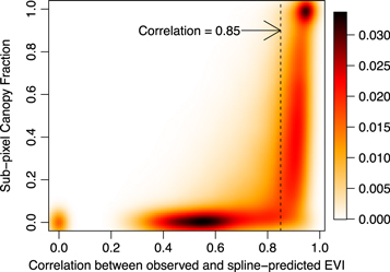
Figure 2. Smoothed scatter plot of sub-pixel canopy fraction versus Pearson correlation coefficients between observed and spline-predicted EVI for pixels within Boston; darker colors correspond to increased density of observations (i.e., higher percentage of pixels located within Boston).
Download figure:
Standard image High-resolution image2.3. Landsat-based surface temperature estimation
Remotely sensed SUHI intensity is widely mapped over various scales using land surface temperature (LST; Yuan and Bauer 2007, Peng et al 2011). For this work, we converted top-of-atmosphere brightness temperatures from the Landsat TM and ETM+ thermal band to LST for all images between May 1 and September 1 using a first-order thermal radiative transfer equation:

where  is the atmospheric transmissivity,
  is the land surface emissivity,
  is the sensor-detected radiance,
  is the target pixel surface radiance, and
  and
and  are the downwelling and upwelling path radiances at the surface and top-of-atmosphere, respectively (Sobrino et al 2004). The radiance values (
 and
and  were converted to brightness temperatures (Tb) using sensor-specific Landsat calibration constants and the inverse Planck equation:
where k1 = 666.09 W m−2 sr−1 μm−1 and k2 = 1282.71 K for Landsat 7 ETM+, and k1 = 607.76 W m−2 sr−1 μm−1 and k2 = 1260.56 K for Landsat 5 TM (Barsi et al 2005). Atmospheric correction was performed using an algorithm based on the MODTRAN5 atmospheric radiative transfer model (Barsi et al 2005; http://atmcorr.gsfc.nasa.gov/), which uses atmospheric profiles of temperature, humidity, and pressure from the National Centers for Environmental Prediction (NCEP) to estimate values for 
 and
and  We ran MODTRAN at 42° N, 71° W and at 15:16 GMT, which to corresponds to the approximate location of Boston and time of the Landsat overpass. Note that because the MODTRAN tool provided by Barsi et al (2005) includes NCEP data extending back to 2000, and the LST data used in this analysis includes imagery from 2000 to 2013.
To prescribe the emissivity at each pixel, we computed area-weighted emissivities based on three sub-pixel land cover constituents (vegetation, bare soil, and urban):
where the  subscript denotes the sub-pixel fraction of urban, vegetation, and soil background within each pixel,
  is the effective emissivity over the Landsat thermal bandpass, and where values for constituent emissivities (εurb = 0.9394, εveg = 0.9740, εsoil = 0.9679) were based on published data (Baldridge et al 2009; see supplementary material). Values of fractional urban land cover,
  were estimated using the Massachusetts Office of Geographic Information's ISA layer (MassGIS 2007), which was generated using 50 cm near infrared orthoimagery and includes all constructed surfaces and man-made compacted soil (i.e., where no vegetation is present). To estimate the fraction of vegetative cover in each pixel,
  we used an approach similar to that used by Carlson and Ripley (1997) and Sobrino et al (2008) (who estimated
  as a function of NDVI), but used EVI because it provides greater dynamic range than the NDVI:
where  (=0.123) and
  (=0.660) were determined using a 1 m spatial resolution map of canopy cover map for Boston (Raciti et al 2014). The fraction of bare soil in each pixel,
  was then calculated as the residual of
  and
and  :
:
This formulation does not include water, which was excluded from the analysis. Further, in contrast to some studies that model sub-pixel cover as a combination of 'high albedo' and 'dark' urban materials (Small 2001, Small and Lu 2006), we assumed that areas located in the  portion of each pixel were uniform in their emissivity.
2.4. SUHI effect on phenology
Our approach for assessing SUHI impacts on green leaf phenology included two main elements. First, to provide a baseline characterization of SOS and EOS patterns across Boston's urban-to-rural gradient, we selected five 50 km transects originating at the Boston Common, a forested park in downtown Boston (figure 1). Two transects were located northeast and southeast of Boston (including some coastal areas), two were located inland to the northwest and southwest, and the fifth transect was located west-northwest of the city. Using these transects, we quantified how the timing of mean EOS and SOS vary as function of (1) distance from the city center and (2) average summertime LST, which we define here as the long-term mean LST based on all available clear-sky observations in May–August (2000–2013).
Second, we explored spatial patterns in SOS and EOS within the city of Boston, focusing on land use and vegetation controls. To characterize urban land use and vegetation cover, we estimated the sub-pixel composition of Landsat pixels within Boston's city limits for each of three surface types: impervious surfaces, tree canopy, and 'other' (grasses, wetlands, fields, bare soil etc). To estimate the fractions of ISA and tree canopy cover, we used the high spatial resolution maps of ISA and tree canopy described in section 2.3. The remaining surface area in each pixel was assigned to the 'other' class (figure 3). As part of this analysis, we also explored if and how two years with unusually cold and warm springs—2003 and 2010, respectively—affected patterns in SOS and EOS in Boston.
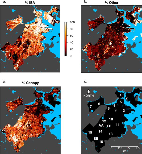
Figure 3. Land use map of Boston, MA where each 30 m pixel is classified as impervious surface area (ISA), forest canopy, or other, based on the within-pixel proportional coverage of each land use class. See table 1 for legend of alphanumeric labels.
Download figure:
Standard image High-resolution image3. Results
3.1. Phenology along urban-to-rural transects
Results from our analysis show that average growing season length (GSL; EOS–SOS) is approximately 18–22 days longer and mean growing season LST is 7 °C higher in urban areas relative to surrounding rural forests, and that spatial patterns in GSL and LST closely follow land use (figure 1). These relationships are consistent across Boston and in nearby cities (e.g., Lowell and Lawrence, located north of Boston in figure 1(a)). GSL is also significantly shorter for wetlands, most of which are located in coastal areas northeast and southeast of Boston.
LST and GSL patterns along the five transects in figure 1 show that relative to nearby rural locations, average SOS occurs about 10–12 days earlier (∼May 5) and EOS occurs about 8–10 days later (∼October 14) in locations that are within about 15 km of the city center (figure 4(a)). However, patterns in SOS and EOS also show substantial local variation (∼4–5 days) caused by heterogeneity in land cover and elevation. In contrast, the relationship between both EOS and SOS as a function of mean growing season LST is smoother (figure 4(b)), but has similar levels of local variation. On average, SOS occurs 1.8 days earlier and EOS occurs 2 days later for each 1 °C increase in mean growing season LST.
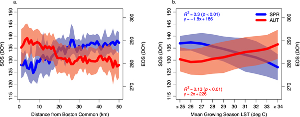
Figure 4. (a) Long-term mean spring (SOS) and autumn (EOS) phenology as a function of distance along five transects drawn from the Boston Common, Boston, MA to outlying rural areas; bold lines represent mean spring and autumn phenology and shaded areas represent ± one standard deviation within 1 km bins. (b) Long-term mean SOS and EOS as a function of mean growing season land surface temperature (LST) along five transects drawn from the Boston Common, Boston, MA to outlying rural areas; bold lines represent mean spring and autumn phenology and shaded areas represent ± one standard deviation within 1°C bins.
Download figure:
Standard image High-resolution image3.2. Relationships between land use and phenology in Boston
Visual analysis reveals strong complementary gradients in ISA and tree canopy cover between northeastern and southwestern Boston, with pronounced local variation. Here we focus on fifteen neighborhoods and three green space areas (table 1, figure 3(d)). In the northeast, Charlestown (1), Downtown Boston (5), and East Boston (2) are heavily developed, but include areas with low stature vegetation (grass, shrubs) in parks along the coast and at Logan Airport in East Boston. Densely residential neighborhoods in Allston (6), Fenway (8), South Boston (3), and the South End (9) have moderate tree canopy cover and relatively high ISA. Lower density residential neighborhoods have much higher overall tree canopy cover, especially in Hyde Park (16), Jamaica Plain (12), and Roslindale (14).
Table 1. Legend of notable parks and neighborhoods within Boston listed in figure 3.
| Symbol | Neighborhood/Park |
|---|---|
| 1 | Charlestown |
| 2 | East Boston |
| 3 | South Boston |
| 4 | Back Bay |
| 5 | Downtown |
| 6 | Allston |
| 7 | Brighton |
| 8 | Fenway/Kenmore |
| 9 | South End |
| 10 | Roxbury |
| 11 | Dorchester |
| 12 | Jamaica Plain |
| 13 | Mattapan |
| 14 | Roslindale |
| 15 | West Roxbury |
| 16 | Hyde Park |
| AA | Arnold Arboretum |
| FP | Franklin Park |
| SB | Stony Brook Reservation |
Long-term mean SOS in Boston ranges from late April to late May (day of year 120–140), and long-term mean EOS ranges from early to late October (day of year 280–290) (figure 5). SOS occurs earlier in neighborhoods such as Jamaica Plain (11) and West Roxbury (15) that have moderate-to-high tree canopy cover mixed with ISA, and later in areas with very dense tree canopy cover such as Franklin Park (FP) and the Stony Brook Reservation (SB). Relative to SOS, spatial patterns in EOS are more variable and show less patch-structure. Spatial variability in both EOS and SOS is highest in neighborhoods such as Dorchester (11) that are the most heterogeneous with respect to tree canopy cover.

Figure 5. Long-term mean (a) spring phenology (SOS) and (b) autumn phenology (EOS) dates within Boston, MA; anomaly in timing of spring onset during (c) 2003 and (d) 2010 within Boston, MA; negative anomalies correspond to earlier than normal arrival in spring.
Download figure:
Standard image High-resolution imageSOS across Boston also shows distinct responses to interannual variation in temperatures. In 2003, for example, the average temperature for February, March, and April at Boston Logan International Airport was 2.9 °C below normal (4th coldest on record). In response, SOS anomalies in 2003 were generally positive (i.e., leaves emerged later than normal) by an average of 4.4 ± 3.4 days (±standard deviation; figure 5(c)). In contrast, temperatures during the same period of 2010 were 4.4 °C above normal (3rd warmest on record) and accumulated growing degree-days were nearly 150% above normal (results not shown). In response, SOS anomalies were uniformly negative (i.e., earlier leaf emergence) by an average of 10.7 ± 4.8 days (figure 5(d)). This effect was most pronounced in areas where average SOS tends to occur later such as the Stony Brook Reservation, where SOS was 15–20 days early in 2010 relative to long-term means.
Finally, to more fully explore the linkage between surface properties and spatial patterns in SOS and EOS, we tested the hypothesis that the amount of ISA in areas surrounding vegetation patches affects local SUHI intensity, and therefore influences the timing of SOS and EOS in urban vegetation patches. Results shown in figure 6(b) appear to confirm this hypothesis: SOS occurs 4.9 days later (t(d.f. = 25 580) = 75.4, p < 0.01) in areas surrounded by land cover with less than 20% ISA relative to locations in more developed areas. In autumn, EOS occurs 0.7 days later on average (t(d.f. = 42 761) = −12.1, p < 0.01) in areas where ISA is greater than 20%, but the relationship is relatively weak (see, figure 6(c)). In 2003 and 2010, pixels surrounded by areas with higher ISA leafed out about 1 day earlier and 2 days later (respectively) relative to normal (figures 6(e) and (f)), which suggests that the influence of ISA and SUHI on spatial patterns in SOS is weaker in years when spring temperatures are anomalous.
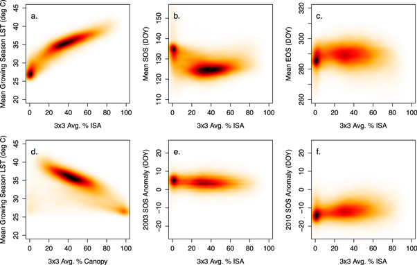
Figure 6. Smoothed scatter plots of a 3 × 3 moving window of percentage impervious surface area (% ISA) within Boston, MA versus (a) mean growing season land surface temperature (LST), (b) mean spring phenology date (SOS), (c) mean autumn phenology date (EOS), (e) 2003 SOS anomaly and (f) 2010 SOS anomaly, and (d) a 3 × 3 moving window of percentage forest canopy within Boston versus mean growing season LST; darker colors in each plot correspond to greater densities of observations.
Download figure:
Standard image High-resolution image4. Discussion and conclusions
Recent research has suggested that UHIs significantly impact the growing season of vegetation in and around cities (Zhang et al 2004, Mimet et al 2009, Krehbiel et al 2016). Our results support this conclusion, but provide a substantially refined characterization of interactions among urban vegetation cover, UHI intensity and vegetation phenology. At regional scales, results from our analysis demonstrate that spring and autumn phenology vary systematically as a function of distance from the center of Boston (or alternatively, with mean growing season LST), leading to growing seasons that are 18–22 days longer within Boston relative to adjacent rural areas. At any specific location, however, the intensity of Boston's SUHI and the average timing of EOS and SOS are both highly variable and depend on local variation in vegetation cover and land use. Hence, spatial patterns in both phenology and SUHI in and around Boston form a tightly linked mosaic that is controlled by local variation in land use (ISA) and land cover (vegetation).
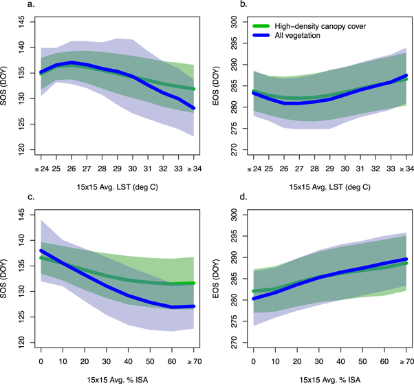
More specifically, results from our analyses demonstrate that the amount of ISA surrounding vegetation patches exert complex controls on SUHI and vegetation phenology. At one extreme, locations such as SB and FP have ISA fractions that are close to zero and have growing seasons that are only slightly longer than adjacent rural areas. Examination of the relationship between SUHI and phenology along a continuum of ISA, however, reveals a clear signature of ISA and SUHI on phenology. For example, figure 7 shows how SOS and EOS vary as a function of average ISA across 15 × 15 pixel moving windows for the entire study region. Here, we use the long-term average wintertime and peak summer EVI to identify pixels with low-density canopy cover and high-density ISA. Pixels with high-density canopy cover have significantly higher average wintertime EVIs (see supplementary material). Using a threshold of wintertime EVI ≥ 0.15 and peak summertime EVI ≥ 0.60, we masked out low-density canopy pixels. Using this, we assessed the impact of urbanization on SOS/EOS separately for (1) all vegetated pixels (including street trees) and (2) only high-density canopy pixels. As figure 7 illustrates, the phenology of high-density canopy pixels was less sensitive to urbanization during spring and equally sensitive during autumn. In areas where the 15 × 15 pixel spatial average LST was greater than or equal to 34 °C, the average timing of SOS was 3.8 days later (t(d.f. = 20 917) = −98.6, p < 0.01), and in areas where the spatial average ISA greater than or equal to 70%, the average SOS was 4.5 days later (t(d.f. = 74) = −7.6, p < 0.01).
Figure 7. (a) Long-term mean spring phenology (SOS) of all vegetated pixels (blue) and exclusively high-density canopy cover pixels (green) as a function of 15 × 15 moving window average land surface temperature (LST); bold lines represent mean spring and autumn phenology and shaded areas represent ± one standard deviation within 1 °C bins. (b) Long-term mean autumn phenology (EOS) as a function of LST. (c) Long-term mean SOS as a function of 15 × 15 moving window average impervious surface area (ISA); bold lines represent mean spring and autumn phenology and shaded areas represent ± one standard deviation within 10% ISA bins. (d) Long-term mean EOS as a function of ISA.
Download figure:
Standard image High-resolution image
Neighborhoods located in Boston's urban core were characterized by higher temperatures, longer growing seasons, and higher proportions of impervious surfaces. In this context, an open question that is not addressed in this paper is the role of species composition in the phenological patterns we observed here. For example, Norway maple (Acer platanoides), a non-native species that is widely found in urban areas of Eastern Massachusetts, leafs out earlier and retains its leaves later than most native tree species that in the region (Bertin et al 2005). Hence, it is likely that at least part of the pattern in GSL that we attribute to Boston's SUHI is also a reflection of geographic patterns in species composition.
Future climate change is expected to have widespread impacts in urban areas. In Boston, general circulation models project that mean springtime temperatures will rise 2.4 °C–6.0 °C by the end of this century (Kirshen et al 2008, McCarthy et al 2010). Results presented here show that in 2010, when spring temperatures were approximately 3 °C above average (i.e., at the low end of projected changes), leaf emergence occurred about 10 days earlier than average in Boston, with trees in Boston's largest forested patches leafing out even earlier. These results are consistent with those of Friedl et al (2014) and suggest that the growing season of trees and urban forests in New England is likely to shift by as much as 2–4 weeks in the coming decades. The full implications of these changes are unclear, but as the Earth's climate warms and urban areas increasingly respond to climate change, urban ecosystems are likely to experience significant functional and structural changes. From a more practical perspective, results from this study show that urban vegetation has the potential to provide significant societal benefit in cities by reducing the intensity of UHIs (Levis and Bonan 2004).
Acknowledgments
We thank Lucy Hutyra and Steve Raciti for providing the canopy layer map and Andy Reinmann, Lucy Hutyra, Brady Hardiman and Leah Cheek for helpful comments and suggestions. This work was partially supported by NASA grant numbers NNX12AM82G and NNX14AI70G, and NSF grant numbers DGE-1247312 and EF-1064614. David Miller participated in the Harvard Forest Summer Program in Ecology, which is supported by the NSF BIO REU program. We gratefully acknowledge support from Harvard and the NSF REU program. We also acknowledge the two anonymous reviewers who volunteered their time to review the manuscript.