


Abstract
The early 21st century was marked by several severe winters over Central Eurasia linked to a blocking anti-cyclone centered south of the Barents Sea. Severe winters in Central Eurasia were frequent in the 1960s when Arctic sea ice cover was anomalously large, and rare in the 1990s featuring considerably less sea ice cover; the 1960s being characterized by a low, the 1990s by a high phase of the North Atlantic Oscillation, the major driver of surface climate variability in Central Eurasia. We performed ensemble simulations with an atmospheric general circulation model using a set of multi-year Arctic sea ice climatologies corresponding to different periods during 1966–2012. The atmospheric response to the strongly reduced sea ice cover of 2005–2012 exhibits a statistically significant anti-cyclonic surface pressure anomaly which is similar to that observed. A similar response is found when the strongly positive sea ice cover anomaly of 1966–1969 drives the model. Basically no significant atmospheric circulation response was simulated when the model was forced by the sea ice cover anomaly of 1990–1995. The results suggest that sea ice cover reduction, through a changed atmospheric circulation, considerably contributed to the recent anomalously cold winters in Central Eurasia. Further, a nonlinear atmospheric circulation response to shrinking sea ice cover is suggested that depends on the background sea ice cover.
Export citation and abstract BibTeX RIS

Content from this work may be used under the terms of the Creative Commons Attribution 3.0 licence. Any further distribution of this work must maintain attribution to the author(s) and the title of the work, journal citation and DOI.
1. Introduction
Climate change during the last decades was characterized by a number of peculiarities. First, the decade 2001–2010 featured the highest globally averaged surface air temperature (SAT) in the instrumental record starting in 1850 (Hansen et al 2010). Second, despite unprecedented levels of atmospheric greenhouse gases, especially carbon dioxide (CO2), global surface warming had considerably slowed during the 21st century relative to the preceding decades. However, third, Arctic average SAT did not depict such a hiatus (Bekryaev et al 2010) and was accompanied by the accelerated Arctic sea ice decline (e.g. Katssov et al 2010).
Another puzzling observation during the recent years was the winter (December through February, DJF) surface cooling over Central Eurasia (figure 1(d)) that was linked to an anti-cyclonic sea level pressure (SLP) anomaly centered to the south of the Barents Sea (figure 1(a)). The temperature evolution is illustrated by the station SAT data of Moscow during 1950–2013 shown for each winter by the DJF average (figure 2). Deviations from any externally-forced long-term climatic trends can be caused by internal atmospheric variability. On interannual timescales, the major driver of SAT variations over Northern Eurasia is the North Atlantic Oscillation (NAO), with anomalously warm (cold) conditions over Central Eurasia linked to a high (low) NAO index. During the recent rather cold years, however, only the anomalously cold winter of 2010 was marked by an extremely low NAO index (figure 2). This, together with the global surface warming pattern during the last decades of the 20th century exhibiting most warming in winter and over the northern continents, which is in line with the average climate model response to observed anthropogenic forcing, made the recent anomalously cold winters over Central Eurasia so surprising.

Figure 1. NCEP winter (DJF) SLP (hPa, upper row) and SAT (°C, lower row) anomalies 2005–2012 (a)–(d), 1990–1995 (b)–(e) and 1966–1969 (c)–(f) relative to 1971–2000.
Download figure:
Standard image High-resolution image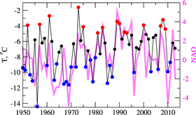
Figure 2. Winter (DJF) surface air temperatures in Moscow (°C, black line) and North Atlantic Oscillation index (thick magenta line). The correlation between the time series is 0.59. The blue and red dots mark strong negative and positive SAT anomalies correspondingly.
Download figure:
Standard image High-resolution imageLet us further illustrate the SAT evolution since 1950 by station data from Moscow (figure 2). The recent harsh winters can be considered as 'normal' when comparing them with those during 1950–1970 (figure 2), indicating strong decadal to multidecadal SAT variability. Predominantly mild winters were observed during 1988–2002. Only one 'cold event' has happened in that relatively warm period, whereas there have been four such events during 2003–2012 and a similar frequency of 'cold events' during 1950–1970 (figure 2). The anomalously warm winters of the 1990s were linked to an exceptionally high NAO index phase, whereas 1960s were characterized by the largest negative decadal NAO index anomaly during the 20th century (e.g. Semenov et al 2008). As pointed out above, the recent anomalously cold years cannot be attributed to a negative NAO index (figure 2). How can we explain these differences? What are the relative influences of the NAO and boundary forcing, specifically Arctic sea ice variability, in driving Central Eurasian SAT during the recent decades?
Negative SAT anomalies over Central Eurasia during the recent years were accompanied by positive SAT anomalies in the Arctic with strongest warming in the Barents Sea region (figure 1(d)), suggesting a possible role of anomalous sea ice extent. In fact, observational analyses have suggested that reduced sea ice concentration (SIC) and cooling over Eurasia were related (Hopsch et al 2012, Outten and Esau 2012, Jaiser et al 2012, Tang et al 2013, Cohen et al 2014, Kim et al 2014). However, the robustness of these results can be questioned given the short observational record. A way out of this dilemma is to study the sea ice variability influence on the atmospheric circulation in an atmospheric general circulation model (AGCM) forced by observed SIC anomalies. Such model simulations provide sufficiently large statistical samples and enable identification of sea ice effects on the atmospheric circulation in the presence of internal variability.
The impact of decreasing Arctic sea ice cover on the atmospheric circulation has been intensively studied with AGCMs (e.g. Alexander et al 2004, Deser et al 2004, 2007, 2010, Honda et al 2009, Petoukhov and Semenov 2010, Lim et al 2012, Rinke et al 2013, Screen et al 2013, Peings and Magnusdottir 2014). A variety of processes has been proposed by which the atmosphere can be impacted including local convection, changed baroclinicity, lower troposphere heating and moistening, and their interaction with large-scale circulation patterns and planetary wave propagation (see Vihma 2014 for review). The atmospheric winter circulation can be either forced by concurrent winter sea ice anomalies (e.g. Alexander et al 2004, Deser et al 2004, 2007, Petoukhov and Semenov 2010) or by sea ice anomalies during the preceding season through delayed feedbacks involving ocean memory or a chain of dynamical processes in the atmosphere (e.g. Cohen et al 2007, 2012, Sokolova et al 2007, Honda et al 2009, Rinke et al 2013, Peings and Magnusdottir 2014). Mori et al (2014) demonstrated a robust winter Eurasian surface cooling as a response to composite SIC anomalies based on high and low September SIC during 1979–2012, supporting previous results by Honda et al (2009).
The atmospheric circulation response to Arctic sea ice variability in models participating in the Coupled Model Intercomparison Project Phase 5 (CMIP5) is rather uncertain (Woolings et al 2014), which, in part, may be related to high uncertainty of the forcing in the Barents Sea region (Smedsrud et al 2013). But what is the role of nonlinearity in the atmospheric response, a critical issue, as many models suffer from large biases? Petoukhov and Semenov (2010) hypothesized that the atmospheric circulation response to an idealized gradual SIC decrease in the Barents and Kara Seas could be essentially nonlinear, with Eurasian surface cooling in response to both anomalously high and low SIC. Indications for such a nonlinearity have been also found by Yang and Christensen (2012) who analyzed the SAT response in the CMIP5 models. Here we present a series of dedicated experiments with a relatively high-resolution AGCM in order to obtain further insights about the atmospheric circulation response to Arctic sea ice variability during the past decades.
2. SIC and atmospheric circulation changes during the past decades
The Greenland Sea and Barents Sea (including the western part of the Kara Sea) are those regions in the Arctic which depict the strongest interannual to decadal SIC variability in winter. SIC changes in these two regions exhibited very different behavior during the past decades. The Barents Sea SIC (figure S1(a)) depicted a rather linear decline until 2004, and thereafter, a fast transition to very low values (marked by red circles in figure S1(a)). In contrast, the Greenland Sea SIC (figure S1(b)) did not feature a long-term trend since the 1980s but exhibited a decline from the late 1960s to the 1980s. Three epochs are highlighted in figures S1(a) and (b): first, the most recent period 2005–2012 which was characterized by very low SIC in the Barents and Greenland Seas (figure 3(c)); second, 1990–1995, a high-NAO index phase (figure 2), which also depicted relatively low SIC in the Barents and Greenland Seas (figure 3(b)); and third, 1966–1969, a low-NAO index phase, which featured high SIC in both Seas (figure 3(a)). The SIC anomalies during 1990–1995 and 1966–1969 are similar in pattern but opposite in sign. Finally, Arctic SIC decline since 1990s was basically confined to the Barents Sea region, with even a small increase in the Greenland Sea (figure 3(d)).
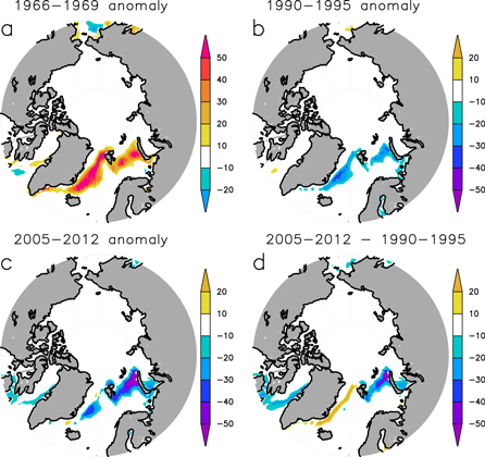
Figure 3. Winter (DJF) sea ice concentration (SIC) anomalies (%) for 1966–1969 (a) 1990–1995 (b) and 2005–2012 (c) relative to the 1971–2000 average SIC. (d) 2005–2012 SIC anomaly relative to 1990–1995.
Download figure:
Standard image High-resolution imageThe corresponding winter SLP and SAT anomalies derived from NCEP reanalysis data (Kalnay et al 1996) depict interesting differences between the three epochs (figure 1). The averaged winter circulation 2005–2012 was characterized by a strong anti-cyclonic SLP anomaly located over and to the south of the Barents and Kara Seas (figure 1(a)), the region where SIC exhibited a step-like decline in 2005 (figure 1(a) and figures 3(c) and (d)). The anti-cyclonic SLP anomaly, which has been observed in 6 winters during that epoch (figure S2), presumably drove the anomalously cold SAT observed over Central Eurasia by blocking the westerly flow and leading to the radiative cooling. The epoch 1990–1995 depicted a typical positive-NAO pattern (Hurrell 1996) with anomalously cold SAT west of Greenland and anomalously warm SAT over most of Eurasia, the Greenland and Barents Seas (figure 1(e)). We also note a strong positive SAT anomaly at the southern border of the Barents Sea, somewhat similar to what was observed during 2005–2012 (figure 1(d)) that may be due to reduced SIC. The epoch 1966–1969 was characterized by a well-defined negative-NAO signal in SLP and SAT over the North Atlantic/Eurasian sector, with conditions that are basically the mirror images of those during 1990–1995 but with much larger amplitude. The epoch 1966–1969 was accompanied by a strong anti-cyclonic SLP anomaly centered south of the Barents Sea (figure 1(c)–(f)), similar to that which has been observed during 2005–2012.
3. Model experiments
The observations suggest that both internal atmospheric variability, specifically that linked to the NAO, and Arctic SIC changes may have acted jointly to drive the atmospheric anomalies over Central Eurasia during the past decades. In order to better understand the SLP and SAT changes described above, a series of ensemble integrations was conducted with the ECHAM5 AGCM (Roeckner et al 2003) forced by sea ice anomalies representing the conditions during the three epochs discussed above. The model employs a horizontal resolution of T106 (1.13° by 1.13°) and 31 vertical levels. Versions of the ECHAM5 AGCM have been previously used for studying the atmospheric response to sea surface temperature (SST) and sea ice anomalies (e.g. Seierstad and Bader 2009, Petoukhov and Semenov 2010, Semenov et al 2012, Semenov and Latif 2012). SST and SIC have been specified from HadISST1 (Rayner et al 2003). A reference experiment was conducted using monthly SST and SIC climatology for 1971–2000. Additionally, three sensitivity integrations were performed. The sensitivity integrations employ the same SST as the reference experiment but use SIC climatologies calculated for the three epochs 1966–1969, 1990–1995 and 2005–2012 (figure 3). Each of these runs is 50 years long with repeating SST and SIC annual cycles for the corresponding epochs. Furthermore, in order to elucidate the role of summer SIC anomalies, a simulation was performed only employing the SIC climatology of 2005–2012 during November through April (the other months have the same SIC climatology as the reference simulation). Atmospheric greenhouse gases and aerosols have present-day values in all simulations, with a CO2 concentration of 348 ppm. We present 50 year averages of winter (DJF) anomalies from the sensitivity integrations with respect to the reference experiment. Statistical significance was estimated by a double sided Student t-test.
4. Model results
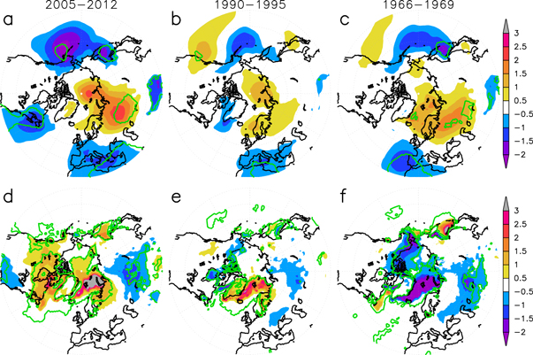
A remarkable feature of the SLP response when driving the model with the SIC anomalies of 2005–2012 is the strong anti-cyclonic SLP anomaly over the Barents Sea region and Central Eurasia (figure 4(a)) which is very similar to what has been observed (figure 1(a)). This anomaly, exceeding 2 hPa in its center, is about a half as strong as the observed and statistically significant at the 95% level, suggesting a significant contribution from Arctic sea ice retreat to the observed circulation change. The anti-cyclonic anomaly is simulated in all three winter months depicting the strongest amplitude in December and January. The probability of positive SLP anomalies south of the Barents Sea in DJF exceeding one standard deviation increases by more than twice (figure S3). Also consistent with observations, the anti-cyclonic SLP anomaly is accompanied by (statistically significant) negative SLP anomalies centered over the Mediterranean region and western North Atlantic. The simulated strong negative North Pacific SLP anomaly is inconsistent with data. This difference may be due to equatorial Pacific SST forcing (Kosaka and Xie 2013) which has not been considered in the model. Statistically significant cooling is simulated over Central Eurasia where strongest anomalies reach −1.5 °C (figure 4(d)). A statistically significant warming is simulated over the Arctic Ocean and northern Canada. The overall SAT response to the SIC change during 2005–2012 is largely consistent with observations and fits the 'warm ocean-cold continent' pattern that has been previously linked to negative SIC anomalies (e.g. Hopsch et al 2012).
Figure 4. Simulated winter (DJF) SLP (hPa, upper row) and SAT (°C, lower row) anomalies in the sensitivity experiments with SIC anomalies for 2005–2012 (a)–(d), 1990–1995 (b)–(e) and 1966–1969 (c)–(f). Anomalies are calculated relative to reference climate simulation using mean conditions 1971–2000. Regions with statistically significant (at the 95% confidence level) differences are denoted by green contours.
Download figure:
Standard image High-resolution image
We now turn to the model response to the moderate 1990–1995 SIC anomalies. The simulated SLP anomalies, somewhat projecting on the negative-NAO pattern, are relatively weak and in general not statistically significant (figure 4(b)). This suggests that the SLP anomalies have been primarily due to internal, i.e. NAO-related variability. The SAT response exhibits statistically significant warming only over the regions of sea ice loss (figure 4(e)) where the observations depict warming too (figure 1(e)). Further, the model's SLP response to the moderate negative SIC anomaly (figure 3(b)) tends to oppose the prevailing positive-NAO pattern during that time, indicating a negative feedback, consistent with results of previous modeling studies which used observed SIC changes prior to the 2000s (e.g. Alexander et al 2004, Deser et al 2004, 2007).
The SLP response to the strongly enhanced SIC during 1966–1969 (figure 4(c)) is similar to that to the strongly reduced SIC in 2005–2012 (figure 4(a)), in the sense that they both feature an anti-cyclonic SLP anomaly south of the Barents Sea, which is consistent with observations (figure 1(c)). The model simulates a cyclonic SLP anomaly centered to the west of the Iberian Peninsula and in the northern North Pacific which are both statistically significant. The North Pacific SLP anomaly is inconsistent with observations but again could be due to the lack of equatorial Pacific SST forcing. The model's SLP response projects on the negative-NAO pattern, suggesting a positive feedback on the atmospheric circulation during 1966–1969. The model fails to simulate the very strong positive SLP anomaly centered over Greenland (figure 1(c)) though reproducing some statistically significant SLP enhancement over the Greenland Sea. The SAT response 1966–1969 resembles the observed change (figure 1(f)) depicting anomalously cold surface temperatures over Central Eurasia, the inner Arctic and Alaska, and anomalously warm surface temperatures southwest of Greenland (figure 4(f)). This pattern can be described as 'cold Arctic-cold continent' as opposed to the 'warm Arctic-cold continent' pattern obtained in the 2005–2012 simulation.
The circulation response presented in figure 4 is generally equivalent-barotropic with height (figure S4), which is in line with the results of previous studies (e.g. Alexander et al 2004, Deser et al 2004, 2007). The strongest height anomalies are, however, located not over the heating area but to the south of the Barents Sea, indicating a dynamical rather than thermodynamical response.
Finally, the simulation only using the 2005–2012 SIC climatology during November through April shows a very similar response pattern (figure S5) with a significant SLP increase south of the Barents Sea. This suggests a major role of winter SIC anomalies in the simulated response, whereas early fall SIC anomalies are of less importance in our model.
The important new result from our forced atmosphere model integrations can be summarized as follows: while the atmospheric response to reduced Arctic sea ice during 1990–1995 is weak, hardly significant and tends to damp the prevailing positive-NAO pattern over the North Atlantic, the stronger amplitude sea ice cover anomalies in 2005–2012 and 1966–1969 tend to reinforce and thus contribute to the atmospheric circulation anomalies, constituting a positive feedback.
5. Discussion and conclusions
This study suggests that anomalously low wintertime Arctic sea ice cover during 2005–2012, which was especially characterized by a strong sea ice loss in the Barents Sea, may have been responsible for the observed anti-cyclonic circulation anomaly centered south of the Barents Sea (figure 2(a)) which was linked to anomalously low SAT over Central Eurasia. Further, we find evidence for the atmospheric circulation response to sea ice cover anomalies during the period of modern sea ice decline is essentially nonlinear, both with respect to amplitude and pattern. Previous work suggested that the atmospheric response to North Atlantic SST and Arctic sea ice anomalies scales linearly with amplitude and nonlinearly with polarity (Deser et al 2004, Magnusdottir et al 2004). Our model results, based on specifying observed SIC changes, suggest that the atmospheric response may also nonlinearly depend on the amplitude of the imposed SIC anomalies.
A possible explanation for the nonlinear atmospheric response was proposed by Petoukhov and Semenov (2010) on the basis of a conceptual model involving the counter play of local convection with thermal wind effect that could explain nonlinearity in the SLP response to gradually reduced SIC in the Barents Sea. We note a large-scale barotropic response structure indicative of planetary wave effects that, in particular, may be responsible for the NAO-like response (e.g. Nakamura et al 2010). Recent studies (Kim et al 2014, Nakamura et al 2015) suggest an important role of troposphere-stratosphere coupling in weakening the stratospheric polar vortex in response to the late fall sea ice retreat that is followed by a negative AO/NAO-phase. In our AGCM, the free troposphere DJF-response to the recent sea ice loss in 2005–2012 also projects on the negative AO-phase (figure S4). However, the strong SIC anomalies of 2005–2012 (and 1966–1969) result in more localized response patterns over and south of the Barents Sea.
We hypothesize that the special character of the SIC anomalies during 2005–2012, which have been much stronger and basically localized only in the Barents Sea in comparison to those during 1990–1995, is responsible for some of the conflicting results outlined above. The SIC anomalies during 2005–2012 are rather different to those expected from long-term trends and to those previously used in AGCM studies. Our findings are supported by recent empirical analyses of the thermal effect due to winter sea ice retreat. Decreased layer thickness gradient reduces zonal flow and stretches stationary planetary wave ridges giving rise to a more meridional circulation with higher probability of blocking events (e.g. Overland and Wang 2010, Francis and Vavrus 2012). It should be noted that such a mechanism may not apply to the response to the enhanced SIC in the 1960s.
Despite some similarities to observations, our model results differ notably from the data. This is not surprising, since the model patterns only represent the response to Arctic SIC anomalies which themselves may partly result from a changed atmospheric circulation. The atmospheric circulation, specifically the NAO, could have experienced strong internal and presumably unpredictable low-frequency variations (e.g. Semenov et al 2008). For example, when linearly removing the NAO-related SAT changes from observations, a cooling pattern emerges during 2005–2012 that is more in line with our model response (Cohen et al 2012). Finally, SST changes, tropical and/or extra-tropical, may also have played a role in influencing the atmospheric circulation in the mid- and high latitudes during the past decades (e.g. Bader and Latif 2003, Hoerling et al 2004, Sutton and Dong 2012, Kosaka and Xie 2013).
Our results are important for understanding the impact of diminishing Arctic sea ice cover on the atmospheric circulation. They are also relevant to understand possible feedbacks between sea ice, ocean and atmosphere in the Barents Sea region that may play a very important role in interannual to decadal climate variability in the Arctic climate system and possibly beyond (Bengtson et al 2004, Semenov et al 2009, Smedsrud et al 2013), and give rise to multi-year predictability over the northern continents.
The nonlinear nature of the atmospheric response to Arctic SIC anomalies found in our model experiments and previously suggested by idealized numerical experiments and CMIP model data analysis may be crucial to understanding the recent cold weather extremes over Central Eurasia. Climatic tendencies such as decrease of subseasonal SAT variability and cold extremes over the Northern Hemisphere observed over the past decade and projected by the CMIP5 models during the 21st century (Screen 2014) do not contradict the opposite tendencies discussed here, as the short-term subseasonal behavior may markedly differ from the longer-term seasonal behavior, as the latter may involve coupled feedbacks.
Acknowledgments
We would like to thank the two anonymous reviewers for their valuable comments. This work was supported by the EU-NACLIM and BMBF-RACE projects, NordForsk GREENICE project, Russian Ministry of Education and Science (contract 14.В25.31.0026), and Russian Foundation for Basic Research (14-05-00518). The model runs were performed at the Northern Germany High‐Performance Computing Center (HLRN).