


Abstract
Heat waves are the most significant cause of mortality in the US compared to other natural hazards. Prior studies have found increased heat exposure for individuals of lower socioeconomic status in several US cities, but few comparative analyses of the social distribution of urban heat have been conducted. To address this gap, our paper examines and compares the environmental justice consequences of urban heat risk in the three largest US cities: New York City, Los Angeles, and Chicago. Risk to urban heat is estimated on the basis of three characteristics of the urban thermal landscape: land surface temperature, vegetation abundance, and structural density of the built urban environment. These variables are combined to develop an urban heat risk index, which is then statistically compared with social vulnerability indicators representing socioeconomic status, age, disability, race/ethnicity, and linguistic isolation. The results indicate a consistent and significant statistical association between lower socioeconomic and minority status and greater urban heat risk, in all three cities. Our findings support a growing body of environmental justice literature that indicates the presence of a landscape of thermal inequity in US cities and underscores the need to conduct comparative analyses of social inequities in exposure to urban heat.
Export citation and abstract BibTeX RIS

Content from this work may be used under the terms of the Creative Commons Attribution 3.0 licence. Any further distribution of this work must maintain attribution to the author(s) and the title of the work, journal citation and DOI.
1. Introduction
In the past two decades, several high mortality heatwave events have been recorded in developed countries. A 2003 heatwave in Western Europe lead to an estimated 50 000–70 000 excess deaths (Robine et al 2008). In 2010, a heatwave combined with atmospheric pollution caused by fires in the Moscow region of the Russian Federation caused an excess mortality of over 11 000 (Shaposhnikov et al 2014). While these events were region-wide in scope, the 2003 heatwave affected densely populated urban areas like Paris, France, and its suburbs which suffered the highest rates of mortality (Fouillet et al 2006). The urban heat island (UHI) effect is the result of several complex factors, including higher structural density and lower amounts of vegetation in urban areas, which create an urban microclimate that is generally hotter than surrounding rural areas (Oke 1992). The relationship between the UHI and elevated mortality has been documented by prior studies (Buechley et al 1972, Clarke 1972, Smoyer 1998). Additionally, higher rates of heat related mortality have been linked with levels of urbanization and acclimatization, as indicated in an analysis of 50 cities of the US (Medina-Ramón et al 2007).
The US is a highly urbanized nation with almost 81 percent of its population living in cities and towns (US Census 2010). This high rate of urbanization increases risks from heat waves for densely situated populations impacted by local climate factors such as the UHI. Urban heat, compounded by periodic and region-wide heat wave events, leads to elevated rates of morbidity and mortality in US cities (Kalkstein and Greene 1997, McGeehin and Mirabelli 2001, Sheridan et al 2008, Zanobetti and Schwartz 2008). Heat waves are currently the most significant weather-related cause of mortality in the US (NOAA, NWS 2013). Several high mortality events in the US provide examples of the devastating effect of heat waves on urban populations during 1980, 1988, 1995, and 1999. The 1995 Chicago heat wave has been the subject of extensive analysis that found socially vulnerable people, which includes low income, elderly, African–American, and/or socially isolated residents, to be disproportionately exposed (Semenza et al 1996, Klinenberg 2002). Subsequent studies of different urban areas of the US have confirmed a linkage between urban heat exposure and factors of social vulnerability (McGeehin and Mirabelli 2001, O'Neill et al 2003, Uejio et al 2011). Because of the seeming inequitable exposure to the risk posed by urban heat on racial/ethnic minorities and economically disadvantaged populations, the problem is beginning to be framed as an environmental justice issue, specifically one of climate justice.
The environmental injustice implications of exposure to urban heat for individuals of lower socioeconomic status were first discussed in Klinenberg's (2002) sociological analysis of the 1995 Chicago heatwave. This association between heat exposure and social vulnerability was explored in more detail by Harlan et al's (2006) quantitative research on 'heat-related health inequalities'. Jenerette et al (2011) expanded this work to emphasize the role of land use and land cover in influencing thermal spatial structure and the development of distinct neighborhood microclimates. These neighborhood level thermal patterns are elements of an 'urban heat riskscape' associated with racial/ethnic minority and lower socioeconomic status. Subsequent research by Chow et al (2012) examined the 'spatial distribution of vulnerability' using a wider range of demographic and socioeconomic variables, but focused on the same urban area (Phoenix, Arizona), as Harlan and Jenerette (2006, 2011). Using data related to heat exposure and other climate-based risk factors in conjunction with an expanded set of variables representing socioeconomic status, Grineski et al (2012, 2013) examined the bi-national sister cities of El Paso and Ciudad Juarez to find social inequities in exposure to climate change in a study area extending across national boundaries of the US and Mexico, respectively. Both these studies extend the concept of the 'climate gap' (Shonkoff et al 2009, Grineski et al 2012, 2013) by which racial/ethnic minority or lower socioeconomic status residents are both inequitably exposed to climate change and possess inadequate resources to mitigate or adapt to its adverse effects.
The environmental justice concerns outlined in the previously discussed research have been expanded in recent work, but most heat-related studies focus on the US Southwest. The largest US metropolitan areas that are often characterized by higher proportions of African–Americans have not been investigated in this research. While some urban heat studies have been conducted outside the US Southwest (McGeehin and Mirabelli 2001, O'Neill et al 2003, Uejio et al 2011), these scholars have not explored the climate justice dimension, or attempted to compare urban areas from different regions of the US. A comparative analytical framework that includes a broader range of socially vulnerable groups and allows generalizations across the various urban heat studies is lacking. A systematic and comparative analysis of large urban areas in the US is necessary to provide a foundation for evaluating the association between elevated urban heat and the location of socially vulnerable populations, and enhance our understanding of the socio-spatial consequences of excess heat exposure.
This article contributes to the emerging environmental justice literature on heat-related inequities by evaluating the spatial and social distribution of urban heat in the three largest US cities: New York, New York; Chicago, Illinois; and Los Angeles, California. By using an index of landscape-related factors collectively related to elevated urban heat, the spatial patterns of association with specific socio-demographic characteristics are examined at the neighborhood level. The objective is to determine if racial/minorities and socioeconomically disadvantaged residents in these three cities are distributed inequitably with respect to an urban heat risk index (UHRI), developed by combining three characteristics of the urban thermal landscape: land surface temperature, vegetation abundance, and structural density of the built urban environment. Our use of a single risk indicator that combines three heat-related variables allows us to better develop and evaluate a comparative framework for analyzing patterns of heat-related inequities than what has been previously done. Statistical associations between this UHRI and multiple indicators of social vulnerability are examined and compared to determine how the socio-spatial distribution of urban heat varies across the three largest cities of the US.
2. Data and methods
The three study areas were selected based on their large population size and the future risk posed by global climate change. The three most populous metropolitan areas in the US were chosen for analysis: New York City, Los Angeles, and Chicago. Climate change modeling based on the Intergovernmental Panel on Climate Change A2 emissions scenario using National Center for Atmospheric Research mid-century (2045–2059) climate models (NCAR/UCAR CESM 2013) indicate that all three cities may be substantially impacted in the future by increasing temperatures, with temperature anomalies ranging from 2.0° to 3.0 °C. The basic unit of analysis for this study are census tracts defined by 2010 Decennial US Census boundaries. Census tracts are one of the basic spatial units of US census enumeration that are commonly used to represent neighborhoods and include a population that ranges from 2500 to 8000 residents. Geographic boundaries for each study area were delineated by selecting contiguous areas of 75% impervious surface, and then including all census tracts within the counties containing those areas of higher ISA. These study area boundaries are depicted in figure 1, which shows that the counties still include urban and suburban areas of their respective cities.
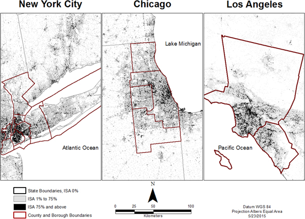
Figure 1. The spatial distribution of percent impervious surface area greater than 75%.
Download figure:
Standard image High-resolution imageHigher percentages of impervious surface area (% ISA) have been used in prior studies as an indicator of urban land uses (Lu and Weng 2006) and urban cores have been defined as areas with greater than 75% ISA (Imhoff et al 2010). For this study, areas of high % ISA were identified using the 2006 National Land Cover Dataset (NLCD 2006) before county boundaries were selected. This technique defines the spatial extent of urban areas through their impact to the landscape, rather than arbitrarily selecting the areas included in US Census Metropolitan Statistical Area boundaries.
This study emphasizes the interaction of physical factors related to urban heat and social vulnerability at the neighborhood level to assess environmental injustice. Landsat Thematic Mapper (TM) remote sensing derived data is used to quantify the physical factors of structural density, vegetation abundance, and temperature. Use of Landsat data allowed for the representation of urban heat at moderate spatial resolutions of 30–120 m, which are sufficient for neighborhood level measurements. The dependent variable in this study denotes the physical aspects of urban heat-related risk, while the independent variables represent the demographic and socioeconomic characteristics of residents in our study areas.
2.1. Dependent variable
A quantitative index of biophysical factors related to urban heat, referred to as the UHRI, was developed and used as the dependent variable for our statistical analysis. The values were estimated using the equation:

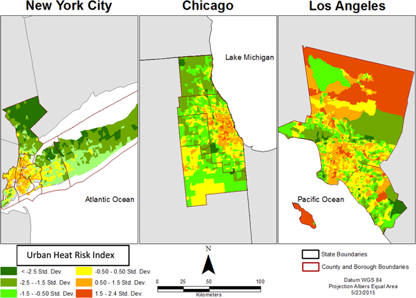
where LST is land surface temperature, NDBI is the normalized difference built-up index which assesses built structure density, and NDVI the normalized difference vegetation index, which is an indicator of vegetation abundance. Prior studies have indicated strong correlations between landscape factors of NDBI and NDVI and the UHI (Xiao-Ling et al 2003, Dousset and Gourmelon 2003). LST, in particular, has been used to delineate the spatial extent of the surface UHI (Voogt and Oke 2003). Additionally, LST has been shown in previous research to have a positive statistical association with rates of heat-related morbidity and mortality (Johnson and Wilson 2009, Johnson et al 2009, Hondula et al 2012). We used the equal weighting approach because there was no logical reason to assume that one of these factors contributes differently to urban heat exposure. The values of LST, NDBI, and NDVI for each pixel in the study areas were derived using Landsat satellite TM 5 remotely sensed imagery. A single clear-sky image from the summer of 2010 was selected for each of the study areas which provided the maximum atmospheric temperature of the available images. In the case of LST, the mono-window algorithm based on the thermal radiance transfer equation was used to extract temperature values from the imagery data (Qin et al 2001, Pu et al 2006). LST, NDBI, and NDVI values were then averaged for the land portion of each census tract, excluding water from calculations of temperature, structural density, and vegetation. The values of these biophysical indicators were then standardized using their z-scores before calculation of the UHRI scores for each tract. The tract level distribution of the UHRI in our study areas is shown in figure 2.
Figure 2. The spatial distribution of the urban heat risk index.
Download figure:
Standard image High-resolution image
2.2. Explanatory variables
The environmental justice consequences of urban heat were assessed with census tract level socio-demographic data from the 2010 US Census and 2009–2013 five-year American Community Survey (ACS) estimates. Our analysis utilizes variables representing extremes of age (children aged five and under and elderly aged 65 and over), race (Non-Hispanic Black and Asian), ethnicity (Hispanic), median household income, educational attainment (percent 25 and over who are high school graduates), and home ownership (owner-occupied homes), with the addition of the Gini coefficient to measure neighborhood level income inequality. The Gini coefficient from the ACS is a summary measure of income inequality that ranges from 0 to 1. A value of 0 indicates perfect equality where all households in a census tract have equal incomes, while a value of one indicates perfect inequality where only one household has any income. This index has been used as a measure of socioeconomic vulnerability and coping capacity in previous EJ studies (Elliott et al 2004, Chakraborty et al 2014). Variables representing the percent of disabled persons (disabled for any reason) and linguistic isolation (percent of households in which no one over 14 yr of age speaks English) were also included. Disability status and linguistic isolation may reinforce social isolation, potentially diminishing the ability of individuals to understand or respond to public health heat warnings and mitigation measures. The variables indicating social vulnerability can then be assessed for their relevance in specific urban and regional contexts using methodologies that are discussed below. Table 1 summarizes the data sources and dates associated with the dependent and independent variables used in the study.
Table 1. Variables used in the study.
| Variable name | Data source | Dates |
|---|---|---|
| Dependent variable: | ||
| Urban heat risk index (UHRI) | Calculated as: (LST + NDVI) − NDBI | Derived from remotely sensed variables below: |
| Land surface temperature (LST) | Landsat 5, TM sensor, 120 meter resolution | New York—4 July 2010; Chicago—10 September 2010; Los Angeles—20 September 2010 |
| Normalized difference built-up index (NDBI) | Landsat 5, TM sensor, 30 meter resolution | |
| Normalized difference vegetation index (NDVI) | Landsat 5, TM sensor, 30 meter resolution | |
| Independent variables: | ||
| % Age 5 and under | US Census | 2010 |
| % Age 65 and over | US Census | 2010 |
| %Non-Hispanic Black | US Census | 2010 |
| % Asian | US Census | 2010 |
| % Hispanic | US Census | 2010 |
| % Disabled | 2013 5 yr ACS estimates | 2009–2013 |
| % High school graduate | 2013 5 yr ACS estimates | 2009–2013 |
| % Non-English speaking | 2013 5 yr ACS estimates | 2009–2013 |
| % Owner-occupied homes | US Census | 2010 |
| Median household income | 2013 5 yr ACS estimates | 2009–2013 |
| Gini coefficient | 2013 5 yr ACS estimates | 2009–2013 |
| Population density | US Census | 2010 |
2.3. Statistical methods
Each study area was analyzed separately using all populated census tracts which were not missing data for any of our explanatory variables. First, descriptive statistics were used to compare the three different study areas. Next, scatterplots of the UHRI and each of our independent variables were examined and natural logarithmic transformations of specific variables were calculated to account for nonlinear relationships. Subsequently, all variable values were standardized and bivariate correlation analysis was conducted using parametric and nonparametric tests, based on Pearson's and Spearman's correlation coefficients.
The relationship between the dependent variable (UHRI) and the set of independent variables in each study area were then analyzed using the ordinary least-squares (OLS) regression method. While OLS regression has been used extensively in the analysis of environmental and social inequities, it assumes that the observations and regression errors are independent. This assumption is likely to be invalid due to the clustering of similar values in space, or spatial autocorrelation (Kissling and Carl 2008, Chakraborty 2011). We tested the residuals for spatial autocorrelation using the global and univariate Moran's I-statistic (Anselin and Bera 1998). The Moran's I for the OLS models associated with all three study areas exhibited significant (p < 001) spatial autocorrelation in the residuals, implying that they failed to meet the assumption of independence. Consequently, we used simultaneous autoregressive (SAR) models, which consider the spatial autocorrelation as an additional variable in the regression equation to estimate its influence simultaneously with that of the other variables (Chakraborty 2011). To determine the appropriate SAR model specification, the Lagrange Multiplier (LM) statistic was utilized (Anselin 2005). The LM test indicated that spatial error models should be used in all three study areas.
Spatial regression models are based on the relationship between neighboring analytical units, using either contiguity or distance between tract centroids to define a spatial weights matrix. Both the queen contiguity approach and iterative selection of distance bands were tested, but the distance-based approach was more successful in reducing residual spatial autocorrelation, as measured by global Moran's I-statistic, to a statistically non-significant level in each study area. The optimal distances for these bands were determined to be 7300, 8500, and 7400 meters, respectively, for New York City, Chicago, and Los Angeles. Finally, the multicollinearity condition index associated with the regression models were found to be smaller than 8.0 in all three study areas, ruling out significant correlations between the independent variables.
3. Results
Differences in the natural and built landscape of each study area greatly impacted the geographic distribution of UHRI scores, particularly in Los Angeles with its sparsely populated desert areas. Visual examination of the spatial patterns of percentage impervious surface over 75% and the UHRI in figures 1 and 2 indicate considerable overlap of these two factors in all three study areas, which should be expected since structural density is one of the variables that comprise the UHRI. However, in the case of Los Angeles, the relationship changes in the extreme northern desert areas that have relatively higher UHRI levels but lower levels of impervious surface. The descriptive statistics for all variables in our three study areas are summarized in table 2.
Table 2. Descriptive statistics for dependent and independent variables.
| New York | Chicago | Los Angeles | |||||||
|---|---|---|---|---|---|---|---|---|---|
| Variable | Min | Max | Mean | Min | Max | Mean | Min | Max | Mean |
| LST(°C) | 22.68 | 51.61 | 44.46 | 25.53 | 35.24 | 31.32 | 30.17 | 53.20 | 45.41 |
| NDBI | −0.194 | 0.233 | 0.081 | −0.094 | 0.209 | 0.062 | −0.020 | 0.338 | 0.138 |
| NDVI | −0.082 | 0.696 | 0.184 | −0.049 | 0.562 | 0.276 | −0.074 | 0.372 | 0.094 |
| UHRI (standardized) | −9.24 | 4.75 | 0 | −7.44 | 5.84 | 0 | −10.76 | 8.66 | 0 |
| % Age 5 and under | 0 | 22.70 | 6.13 | 0 | 16.00 | 6.60 | 0 | 15.20 | 6.42 |
| % Age 65 and over | 0 | 82.60 | 12.77 | 0 | 52.40 | 11.60 | 0.10 | 82.40 | 11.38 |
| % Non-Hispanic Black | 0 | 96.51 | 21.95 | 0.03 | 99.34 | 23.53 | 0 | 90.75 | 7.19 |
| % Asian | 0 | 88.13 | 10.71 | 0 | 88.88 | 5.98 | 0 | 87.20 | 14.28 |
| % Hispanic | 0 | 93.20 | 26.01 | 0.10 | 98.70 | 20.70 | 3.00 | 99.00 | 44.09 |
| % Disabled | 0 | 74.00 | 9.42 | 0 | 36.00 | 9.84 | 0 | 88.20 | 9.23 |
| % High school graduate | 0 | 100.00 | 72.56 | 28.50 | 100.00 | 84.83 | 23.50 | 100.00 | 76.46 |
| % Non-English speaking | 0 | 74.70 | 12.79 | 0 | 53.20 | 7.69 | 0 | 79.10 | 14.99 |
| % Owner-occupied homes | 0 | 100.00 | 45.31 | 0 | 100.00 | 61.71 | 0 | 96.70 | 50.60 |
| Median household income | 9675 | 243 622 | 67 285 | 9550 | 236 250 | 63 840 | 6406 | 231 648 | 64 829 |
| Gini coefficient | 0.0189 | 0.6750 | 0.432 | 0.209 | 0.721 | 0.4204 | 0.060 | 0.720 | 0.415 |
| Population density | 5 | 114 639 | 14 610 | 12 | 196 409 | 4215 | 1 | 36 483 | 4739 |
| Number of tracts | 3096 | 1838 | 2927 | ||||||
Of the three study areas, Los Angeles with its sprawling urban structure and arid region north of the San Gabriel Mountains has the highest mean NDBI, and lowest NDVI, indicating that it is extensively built-up and sparsely vegetated, with areas of exposed rock and soil. One limitation of the NDBI is its inability to delineate areas of barren soil from built urban structure, (Zha et al 2003). Los Angeles also had the highest mean LST and the date that the remote sensing image was taken ( 20 September 2010) coincided with a heatwave in the Los Angeles region during which the daily high atmospheric temperature exceeded 40 °C.
In contrast to Los Angeles, the cities of Chicago and New York are more extensively vegetated and have lower structural density as measured by the NDVI and NDBI. Chicago had the lowest mean LST, the imagery been taken on 12 September 2010, a day when atmospheric temperature reached only 30 °C. Cloud-free Landsat TM imagery taken on a day of warmer atmospheric temperatures was not available for Chicago that year. The data for New York revealed a higher mean NDBI and lower NDVI than Chicago, indicative of greater structural density and less extensive vegetation. New York was also much warmer than Chicago, with a mean LST only 1 °C cooler than Los Angeles. This is because the New York data was taken on 4 July 2010, with a daily high temperature of 35 °C and also because it was a longer summer day, with an hour more insolation at the time of image capture than for either Chicago or Los Angeles. The values of LST, NDBI and NDVI were standardized prior to the calculation of the UHRI variable. In the case of LST, this standardization compensated for differences in temperature levels for the dates the remote sensing imagery was taken. The UHRI scores indicate the highest mean values for New York, followed by Los Angeles and Chicago. This can be partly explained by the very high LST and low NDVI values for tracts in the desert areas of Los Angeles, some of which were excluded from the study due to their low population values of less than 500. LST in the New York study area ranged widely, and landcover varies from marshes to concrete and asphalt, however unlike Los Angeles, the hottest tracts still contained exposed populations. While the landscape of Los Angeles may have greater extremes in temperature and less vegetation, the manner in which its population is exposed to these risks differs from that of Chicago and New York.
Examination of descriptive statistics for the independent variables (table 2) reveals considerable differences in socio-demographic characteristics that reflect the diverse urban ecologies of these study areas. New York City has a much higher population density than the other two study areas, an indicator of the intensity and extent of its residential built urban structure. There are substantial differences in the socioeconomic and racial/ethnic composition of the three cities. Los Angeles has a lower Non-Hispanic Black and higher Hispanic mean population percentages in its tracts than the other cities and also a higher percentage of linguistically isolated households. Chicago had the highest Non-Hispanic Black and lowest Asian mean population percentages, but also the highest mean percentage of high school graduates.
Bivariate correlations of the UHRI scores with the independent variables, listed in table 3, revealed similar statistical relationships across the three study areas for most variables. The age-related variables show consistent significant and positive associations with the UHRI for percentage age 5 and under, and negative for age 65 and over. This limited exposure appears to be inconsistent with prior research which suggests that elderly adults are not only a particularly vulnerable group, but may have higher levels of exposure (Semenza et al 1996, Klinenberg 2002, Fouillet et al 2006). However, socioeconomic status may be a confounding factor since the percentage of individuals aged 65 or more shows a significant and positive relationship with home ownership based on Pearson's correlation coefficient in all three study areas, and with median household income in New York City and Los Angeles. The percentages of Non-Hispanic Black and Hispanic residents are consistently and positively associated with the UHRI, suggesting that tracts with higher proportions of these racial/ethnic groups are exposed to higher levels of biophysical risk. The Asian subgroup indicates a significantly positive correlation only in New York City, but significantly negative relationships in the two other areas.
Table 3. Bivariate correlation of urban heat Risk index with census tract level independent variables.
| Pearson's r | Spearman's ρ | |||||
|---|---|---|---|---|---|---|
| Variable | New York | Chicago | Los Angeles | New York | Chicago | Los Angeles |
| % Age 5 and under | .218** | .328** | .426** | .241** | .354** | .467** |
| % Age 65 and over | −.323** | −.259** | −.416** | −.429** | −.300** | −.467** |
| % Non-Hispanic Blacka | .249** | .216** | .212** | .237** | .250** | .254** |
| % Asiana | .195** | −.076** | −.099** | .116** | −.245** | −.241** |
| % Hispanicb | .222** | .435** | .547** | .213** | .347** | .580** |
| % Disabled | .207** | .157** | .146** | .173** | .151** | .145** |
| % High school graduatec | −.130** | −.505** | −.591** | −.132** | −.532** | −.651** |
| % Non-English speakingd | .430** | .376** | .488** | .468** | .296** | .545** |
| % Owner-occupied homes | −.671** | −.534** | −.442** | −.664** | −.549** | −.472** |
| Median household income | −.541** | −.515** | −.625** | −.530** | −.517** | −.659** |
| Gini coefficient | .175** | .066** | −.181** | .227** | .083** | −.113** |
| Population densitya | .537** | .317** | .357** | .664** | .678** | .402** |
Note: **p < .01Variables natural log transformed: a = Los Angeles, New York; b = Chicago, New York; c = Chicago, Los Angeles; d = Chicago, Los Angeles, New York.
In terms of the other variables, the percentage with a disability shows positive and significant correlations with the UHRI in all three areas. Educational attainment measured by percentage of high school graduates was significantly and negatively associated, while linguistic isolation was significant and positive in all three study areas. Relationships were particularly strong, significant, and consistent between the UHRI and socioeconomic characteristics. Median household income and home ownership show significant and negative relationships with the UHRI, indicating that greater biophysical risk is associated with lower socioeconomic status in all three study areas. Finally, population density is consistently significant and positive across the three study areas.
Table 4 summarizes the results of the spatial error regression analysis (regression coefficients) for the three cities. The percentage of individuals aged 5 and under was significantly and negatively related with UHRI in New York City and Los Angeles, but positively related in Chicago. The significance and direction of relations between UHRI and the variable age 65 and over was significant and negative in New York City and Los Angeles, but non-significant in Chicago. The proportion of racial/ethnic minorities was generally higher in areas of greater urban heat risk. Non-Hispanic Black and Hispanics were significantly and positively related to the UHRI in Chicago and Los Angeles, while Asians were significantly and positively associated with the UHRI in all three study areas. Disability was significant and positive only in Los Angeles, The percentage of high school graduates significant and negative in Los Angeles. Linguistic isolation measured by percent Non-English speaking households was significant and positive in both New York and Chicago.
Table 4. Spatial error regression of urban heat risk index.
| New York | Chicago | Los Angeles | |
|---|---|---|---|
| % Age 5 and under | −.048** | .066** | −.092** |
| % Age 65 and over | −.134** | −.019 | −.111** |
| % Non-Hispanic Blacka | −.013 | .067*** | .095** |
| % Asiana | .031*** | .089** | .169** |
| % Hispanicb | −.111** | .145** | .297** |
| % Disabled | .014 | −.005 | .044*** |
| % HS graduatec | −.007 | −.013 | −.120** |
| % Non-English speakingd | .079** | .068** | .011 |
| % Owner-occupied homes | −.269** | −.019 | −.211** |
| Median HH income | −.076** | −.144** | −.259** |
| Gini coefficient | −.076** | −.135** | −.123** |
| Population densitya | .496** | −.009 | −.229** |
| Spatial error term (rho) | .772** | .960** | .906** |
| Akaike Info Criterion | 5237.82 | 3106.46 | 5567.99 |
| Pseudo r-squared | 0.69 | 0.70 | 0.62 |
| Moran's I | −0.001 | −0.001 | 0.001 |
Note: ***p < .001; **p < .01; *p < .05Variables natural log transformed: a = Los Angeles, New York; b = Chicago, New York; c = Chicago, Los Angeles; d = Chicago, Los Angeles, New York.
The socioeconomic variables generally showed the same consistent patterns of significant and negative associations with the UHRI that were revealed in the bivariate correlation analysis. Home owner-occupancy was significant and negative in New York City and Los Angeles, while median household income showed a significant negative relationship across all three study areas. The Gini coefficient was also significantly negatively associated, indicating greater economic homogeneity for tracts with elevated UHRI. These three factors collectively imply that there is a consistent relationship between lower socioeconomic status and increased UHRI across our study areas.
Our spatial definition of study regions for this analysis relies on the selection of areas with high percentages of contiguous impervious surface and the political boundaries of the associated counties. This approach results in the inclusion of urban, suburban, and sometimes rural areas within the counties selected for analysis. The final step of our analysis focuses on assessing how the statistical relationships with the UHRI observed in table 4 would change if rural and suburban areas with relatively lower population density were excluded from each of the three study areas. To compare the results of the broader metropolitan areas with those of their core urban areas, restricted and more structurally dense areal extents were chosen and spatial regression models were estimated for these core urban areas. The New York City study area was redefined using data from its five boroughs and Hudson County, New Jersey, Chicago was restricted to the boundaries of Cook County, and only areas South of the San Gabriel Mountains were included in the Los Angeles study area. This resulted in the exclusion of rural areas in north Long Island and Westchester County with higher vegetation and low structural density (New York), rural areas north and west of Cook County (Chicago), and the arid and less vegetated northern areas which produce high NDBI values and yet are not structurally dense (Los Angeles). For estimating the spatial error models for these core urban areas, spatial weights were recalculated resulting in 5100, 6000, and 7200 meter distance bands for New York City, Chicago, and Los Angeles, respectively. The regression results for both the larger metropolitan and core urban areas are summarized in table 5. In both Chicago and Los Angeles, the statistical significance and signs for most explanatory variables are similar in the broader metropolitan and core urban areas, although regression coefficients for a few variables indicate higher values. The results for New York, however, reveal substantial changes when the predominantly rural areas are excluded from the analysis. When the more structurally dense and socio-demographically heterogeneous core area is considered, the signs of the coefficients relating the UHRI to the Gini coefficient, median household income, and percent high school graduates all change to become significant and positive, as do the coefficients for the variables percent age 5 and under and percent Hispanic population. Additionally, percent Asian residents becomes non-significant, the percent disabled becomes significant, and home owner-occupancy becomes non-significant in the model for the core area of New York City. These directional changes in statistical associations with the UHRI for eight of our 12 explanatory variables in New York City emphasize the importance of scale and spatial extent when selecting study areas for urban heat analysis. The relatively minor changes in significance of the variables in Chicago and Los Angeles indicates the stability of the UHRI model in those areas, though goodness-of-fit as indicated by the pseudo r-squared and Akaike Information Criterion is reduced in models from the core urban areas when compared to the models based on the larger study area extents for all three study areas.
Table 5. Comparison of spatial error regression model results for broader metropolitan and core urban areas.
| New York | Chicago | Los Angeles | ||||
|---|---|---|---|---|---|---|
| Broader metro | Core urban area | Broader metro | Core urban area | Broader metro | Core urban area | |
| % Age 5 and under | −.048** | .177** | .066** | .421** | −.092** | −.108 |
| % Age 65 and over | −.134** | −.357** | −.019 | −.015 | −.111** | −.229** |
| % Non−Hispanic Blacka | −.013 | −.099 | .067*** | .387** | .095** | .322** |
| % Asiana | .031*** | −.016 | .089** | .315** | .169** | .196** |
| % Hispanicb | −.111** | .328** | .145** | .575** | .297** | .484** |
| % Disabled | .014 | .113* | −.005 | .065 | .044*** | .204** |
| % HS graduatec | −.007 | .398** | −.013 | .0003 | −.120** | −.539** |
| % Non-English speakingd | .079** | .344** | .068** | .179** | .011 | .168** |
| % Owner-occupied homes | −.269** | −.074 | −.019 | .219* | −.211** | −.285** |
| Median HH income | −.076** | .219** | −.144** | −.165 | −.259** | −.567** |
| Gini coefficient | −.076** | .439** | −.135** | .082 | −.123** | −.050 |
| Population densitya | .496** | .498** | −.009 | .082 | −.229** | −.171** |
| Spatial error term (rho) | .772** | .945** | .960** | .957** | .906** | .161 |
| Akaike Info Criterion | 5237.82 | 8803.88 | 3106.46 | 4762.67 | 5567.99 | 10532.50 |
| Pseudo r-squared | 0.69 | 0.49 | 0.70 | 0.61 | 0.62 | 0.49 |
| Moran's I | −0.001 | 0.001 | −0.001 | <.001 | 0.001 | <.001 |
| N (no. of tracts) | 3096 | 2327 | 1838 | 1318 | 2927 | 2638 |
Note: ***p < .001; **p < .01; *p < .05Variables natural log transformed: a = Los Angeles, New York; b = Chicago, New York; c = Chicago, Los Angeles; d = Chicago, Los Angeles, New York.
4. Concluding discussion
The effects of urbanization and an increasing global temperature baseline make cities important sites for studying racial/ethnic and socioeconomic inequities in heat exposure and its negative consequences. There have been recent indications that urban areas have experienced higher incidences of heat waves, with half of the 217 cities in a recent global study showing increases in extreme hot days from 1973 to 2012 (Mishra et al 2015). The current pace of urbanization combined with temperature increases will probably expand the number of people exposed to the adverse health effects of episodic heat waves. In this context, our study focused on documenting and analyzing landscapes of thermal inequity which are developing in the US, but exist at a variety of scales across our planet. The dynamic behind this landscape are the anthropogenic modifications to the land surface by urbanization and chemical composition of the atmosphere through industrialization. This landscape of thermal inequity is influenced by aspects of a physical landscape produced by changes in structural density and vegetation discernible in the UHI effect and its alteration of urban microclimates. It also manifests as a transformation to the landscape due to changes in regional climate resulting in greater temperature extremes and shifting rainfall patterns. Finally, it is also a social landscape of community location and varying urban ecology.
Our study provides a comparative assessment of urban heat exposure resulting from changes to the physical landscape and factors relating to urban ecology which shape the spatial pattern of social vulnerability in the three largest US cities. By developing a new risk index, our research allows the systematic and comparative analysis of urban heat in different cities. There are, however, certain limitations associated with the evaluation of disproportionate heat risk using urban landscape factors. One limitation is that mitigating or adaptive strategies like air conditioning are not accounted for. Most people in urban areas spend a higher portion of their time indoors, which would be mitigated by the presence or absence of air conditioning, which is itself potentially influenced by socioeconomic status. Additionally, the presence or absence of private backyard shade access can also factor into heat risk. Although these variables were not included in our study, these factors might alter the statistical relationships that we found. Synthesizing across the three study areas, we find consistent and significant associations between the risk factors of urban heat and lower socioeconomic status of urban residents, which are similar to those reported in previous studies of other US cities. The greatest consistencies in association were present in the socioeconomic variables related to household income and home ownership, and also the Gini coefficient, while the demographic variables suggest that local patterns in the distribution of racial/ethnic minority neighborhoods influence the relationship between heat exposure and social vulnerability. Higher risk burdens imposed on neighborhoods occupied by African–American and Hispanic residents were consistently evident in the bivariate correlations, and in all areas except New York in the multiple regression analysis. Linguistic isolation was also a significant factor in all areas except for Los Angeles. We also found disproportionate exposure to heat risk for neighborhoods that contain a higher proportion of disabled individuals and those who lack high school education. Our comparison of analytical results from the broader metropolitan and core urban areas indicated that scale and spatial extent of the study area is an important consideration for analyzing thermal inequity. The spatial error model estimated for core urban areas revealed several changes in the results for New York City, but indicated relatively minor changes in the significance and signs of variables for Chicago and Los Angeles. These differences are indicative of the varying urban ecologies of the study areas, as well as their relationships with structural and vegetation density and land surface temperature.
In conclusion, our statistical findings point to a climate justice issue that is related to the 'climate gap' suggesting that people and households with reduced economic means to adapt to and mitigate the effects of urban heat have greater exposure to its adverse effects (Shonkoff et al 2011, Grineski et al 2013). The association between urban heat risk and social vulnerability indicates the need for improved UHI and heat wave mitigation strategies. Since the problem of urban heat exposure is complicated by local factors related to the urban structure and by an increasing global temperature baseline, it demands policy decisions at multiple scales. Structuring effective strategies involves increased research, planning, and resource allocation in areas of cities where minorities and low-income populations are concentrated and more exposed to extreme heat. A major impediment here is the lack of awareness among urban planners and public health officials of the risk burdens imposed on socially vulnerable residents by elevated greenhouse gas and co-pollutant emissions and their amplification by urban heat (Mendez 2015). However, the landscape of thermal inequity found in the three largest US cities represents an important example of climate injustice faced by communities characterized by racial/ethnic minorities and socioeconomically disadvantaged residents and underscores the need to conduct more comparative analyses and develop appropriate policy solutions.