

Abstract
This paper presents a numerical investigation into the aerodynamic characteristics and fluid dynamics of a flying snake-like model employing vertical bending locomotion during aerial undulation in steady gliding. In addition to its typical horizontal undulation, the modeled kinematics incorporates vertical undulations and dorsal-to-ventral bending movements while in motion. Using a computational approach with an incompressible flow solver based on the immersed-boundary method, this study employs topological local mesh refinement mesh blocks to ensure the high resolution of the grid around the moving body. Initially, we applied a vertical wave undulation to a snake model undulating horizontally, investigating the effects of vertical wave amplitudes (). The vortex dynamics analysis unveiled alterations in leading-edge vortices formation within the midplane due to changes in the effective angle of attack resulting from vertical bending, directly influencing lift generation. Our findings highlighted peak lift production at and the highest lift-to-drag ratio (L/D) at , with aerodynamic performance declining beyond this threshold. Subsequently, we studied the effects of the dorsal–ventral bending amplitude (), showing that the tail-up/down body posture can result in different fore-aft body interactions. Compared to the baseline configuration, the lift generation is observed to increase by 17.3% at = 5°, while a preferable L/D is found at = −5°. This study explains the flow dynamics associated with vertical bending and uncovers fundamental mechanisms governing body–body interaction, contributing to the enhancement of lift production and efficiency of aerial undulation in snake-inspired gliding.


Original content from this work may be used under the terms of the Creative Commons Attribution 4.0 license. Any further distribution of this work must maintain attribution to the author(s) and the title of the work, journal citation and DOI.
1. Introduction
Gliding is a type of aerial locomotion that many land-based tropical creatures adapt to maneuver through the forest and reduce the energy cost when traveling. Such enhanced horizontal mobility is obtained by exchanging the potential energy for kinetic energy [1]. As a form of flight, gliding requires animals to generate aerodynamic forces such as lift and drag when airborne [2]. Many gliding animals, like colugos, flying frogs, and butterfly lizards, have adapted their bodies to glide through the air. They have developed wing-like structures such as membranous wings, skin flaps, and flattened bodies to help them glide [3–5]. Unlike animals mentioned above, flying snakes glide through the air by widening their bodies up to two times to generate lift from the airfoil-shaped body cross-section. This body profile has been intriguing to researchers, leading to a few experimental and numerical studies on the corresponding aerodynamic characteristics [6–10].
During the gliding flight, the flying snake body can be treated as a combination of many segments as a result of the traveling wave. While some anteriorly located body segments directly encounter the freestream airflow, some other posteriorly located body segments encounter the flow induced by the upstream segments. This indicates the downstream body parts may interact with the wake of upstream body parts. The location of the downstream body parts is exhibited to be changing with high amplitudes up to 30° during the gliding, as reported in an experimental study by Yeaton et al [11]. Specifically, during the gliding flight, they observed an up–down motion on the posterior body part relative to the head position, termed the 'dorsoventral bending', resulting in different body configurations. However, how the body postures and posterior body location affect the aerodynamic performance is unclear. Miklasz et al [7] approached this question by experimentally arranging two snake-inspired airfoils in tandem configuration to mimic the fore-aft interaction between the anterior and posterior parts of the snake body. In their study, a 26% increased lift production with a 54% enhanced lift-to-drag ratio (L/D) is found on the downstream airfoil as it is located 0.9 chord lengths below and 3 chord lengths apart from the upstream airfoil. The effect of the combinations of spatial arrangements and varied angles of attack (AOA) on the aerodynamic performance was numerically investigated by Jafari et al [12] using a pair of two-dimensional (2D) snake-like airfoils. They found that the performance of a tandem foil system is highly dependent on their relative positions and the AOA, as the L/D could result in the variance between decreasing by 10% to increasing by 12%. They also identified a wake interaction on the trailing airfoil, which allowed for higher lift production. However, the role of the posterior up–down motion in the undulation motion remains unclear. By applying a heaving motion to the downstream snake-like airfoil to simulate the up–down motion in the posterior body, Gong and Dong [13] reported a vortex-capturing mechanism on the downstream airfoil, taking advantage of the upstream wake by higher lift production. The studies above revealed some aerodynamic benefits on the posterior body resulting from wake interaction. However, these findings are constrained in 2D, neglecting the three-dimensional (3D) lateral vortex structures formed in the side-to-side undulation motion. This may overlook the lift-producing mechanisms behind the lateral motion in snake-inspired gliding flight.
Different from other gliding animals with minimal body movements, flying snakes gliding through the air involve large amplitude lateral motions and vertical excursions. Such deformation of the snake has been observed and recorded for a long time. Socha et al [1] have used the location landmarks on the snakes' bodies to document this aerial undulation. The movement is characterized by a horizontal S-shaped traveling wave with high side-by-side amplitudes of up to 34% of the snout–vent length, and this traveling wave develops along the body over time at an average frequency of 1.4 Hz. Socha et al [14] further summarized the displacement of the head and the vent during a non-equilibrium gliding process. From their experiment, they recorded that the body has a large amplitude motion compared with the head, and in the vertical direction the head is usually above the vent. Yeaton et al [11] conducted experiments to measure the snake's posture in the indoor glide arena. Their collective data suggest that the snake's undulation motion can be decomposed into a large-amplitude horizontal wave and a smaller-amplitude vertical wave, thus proposing a mathematical model to describe the wave function. From the observation, the snake tends to have a horizontal undulation amplitude ranging from 85° to 120°, and a vertical bending amplitude ranging from 20° to 45°. Such a model provides us with a more systematic way to study the aerodynamic performance of flying snake gliding, however, these effects have not received significant attention.
The effect of the horizontal undulation motion was recently studied by Gong et al [10] using a 3D flying snake-inspired model to study the lift-producing mechanism. The leading-edge vortex (LEV) tube is identified to be the most crucial element in lift production in flying snakes' gliding, and this mechanism is sturdy across various parameters such as AOA, undulation frequency, and Reynolds number. Furthermore, under the 3D effect, an optimal AOA at 45° is found to produce maximum lift, which is higher than the optimal AOA at 35° found in the previous 2D study [8]. This suggests the presence of a delayed stall in the 3D flow in the flying snake's gliding flight. In previous studies, it was noted that in addition to the characteristic horizontal S-shaped movement, snakes in gliding flight also exhibit vertical wave undulations and dorsal–ventral bending. However, the impact of these additional motions on internal interactions and aerodynamic performance during snake gliding flight remains unknown.
In this study, we aim to deepen our understanding of 3D flying snake gliding by examining the impact of vertical bending motions on aerodynamic performance. Utilizing a 3D snake-shaped model from our previous research [10], we assess these effects through a numerical evaluation of flow features near the body. Our analysis employs a high-fidelity, in-house developed direct numerical simulation (DNS) flow solver. We conduct in-depth investigations into how different vertical bending motions alter the near-body vortex topology and correlate these flow phenomena with performance changes, such as enhanced lift production and improved gliding efficiency. The rest of the paper is organized as follows. Section 2 describes the physical problem and the numerical method used. Section 3 presents the results and discussions in detail, with subsections dedicated to discussing the effects of vertical wave undulation and dorsal-ventral bending. Finally, section 4 provides concluding remarks.
2. Methodology
2.1. Modeling of kinematics
Shown in figure 1(a), the current study employs a flying snake model with polygonal-mesh skin that is bounded to a joint-based hierarchical skeletal structure to control the undulatory motion using the 3D modeling software Autodesk® Maya (Autodesk Inc. Mill Valley, California, U.S.). The undulatory motion is decomposed into joint rotations and is then applied to the joints along the snake body to realize the gliding kinematic. This technique has been successfully applied in previous work [15–17]. The gliding snake kinematic can be decomposed into horizontal undulation and vertical undulation, as reported by Yeaton et al [11]. The horizontal decomposition is realized by applying a horizontal bending angle () to each of the body segments, which has been evaluated in our previous study [10], and the vertical undulation is realized through the vertical bending angle (ψ). The bending angle definitions are illustrated in figure 1(b). It is shown that the horizontal bending angle is always defined in the plane XOZ, indicating the angle between the projection of the body vector and the front direction (−X). The vertical bending angle is the angle between the body vector and the projection vector on the plane.


Figure 1. (a) Skeletal structure for the snake model. (b) Definitions of the horizontal () and vertical () bending angles. (c) Schematic of the skeletal structure that controls the kinematics. stands for the global coordinates of the discrete body segment. is the length of each segment and represents the accumulative arc length of the snake.


Download figure:
Standard image High-resolution imageFigure 1(c) shows the schematics for the skeletal structure that controls the flying snake gliding kinematics. The rotation of each joint is dependent on the local body arc length , and it is approached by the summation of finite numbers of distances between joints. Therefore, the global coordinate for each joint's location can be expressed as:

where represents the coordinate of the kth joint (k = 1, 2, ..., N, where N is the total joint number), represents the segment length between two neighboring joints, and is the unit vector describing joint orientation. The multiplication of represents the displacement added by the jth joint, and the summation adds up to the position of the current joint. Thus, we can calculate the arc length (until the kth joint) of the snake body using the following summation:


The joint direction in equation (1) is described with the following unit vector:

where and represent the horizontal and vertical bending angles of the kth joint at the snake body. These bending angles are defined with the following equations for each joint along the body as a function of time:


Equations (4) and (5) describe the change in horizontal and vertical undulation angles on the kth joint at a given time t, over a motion cycle period of T. and represent the maximum horizontal and vertical bending angle, respectively. , , and are the wave number, undulatory frequency, and phase shift that are related to the horizontal motion; and , and are those related to the vertical motion. is the accumulative body arc length. In the previous study by Gong et al [10], when only considering the horizontal undulation, the optimal aerodynamic performance was found with = 93° and = 1.4°. The current study kept these parameters constant to analyze the impact of vertical undulations. The relation between the horizontal and vertical motion concerning the wave number and undulatory frequency is described as = 2, and = 2, according to [11]. Furthermore, the effect of the dorsal–ventral bending is also studied herein, realized by including an additional term, , to equation (5), which allowed for a vertical offset along the length of the body, .


Figure 2 shows the three-axis-view schematic to describe the setup for the flying snake model with different vertical bending patterns. The head and tail of the model are marked in red and blue dots, respectively. Figure 2(a) presents the model with no vertical motions studied in the previous work [10] as a reference, showing an obvious S-shaped body posture, as mentioned previously. The baseline case to study the effect of vertical wave undulation is set to be = 10° and = 0°, with the corresponding configuration displayed in figure 2(b). The top view reveals a relatively unchanged S-shaped body posture compared to that in figure 2(a). Moreover, the front view in figure 2(b) shows an '8' shape on the snake's body that is introduced by the vertical bending angle , compared to the pure flat body configuration with no as shown in the front view from figure 2(a). The side view also shows a neutral position of the model with no dorsal–ventral bending. Figure 2(c) shows the configurations considering the dorsal–ventral bending with a maximum amplitude of = 5° and −5°. The top views remain similar to the previous configurations due to the control factors for the side-to-side undulation motions remain unchanged. However, the side views in figure 2(c) show the tail-down/up motion that resembles a body tilting motion controlled by the dorsal–ventral bending amplitudes . Specifically, a positive results in a tail-down motion, while a negative results in a tail-up motion as shown in figure 2(c). The parameters that we investigated through the whole research are listed in the table:


Figure 2. Three-axis-view schematics of the flying snake model under different parameters. Red and blue circles indicate the head and tail tip of the model. The configurations are (a) without vertical wave undulation ( = 0°), and (b) with a vertical wave undulation amplitude at = 10°. (c) The dorsal-ventral bending amplitudes at = 5° and −5° are applied to the configuration in (b).


Download figure:
Standard image High-resolution imageAccording to the experimental report [11], the vertical undulation can reach the amplitude of 45° and the dorsal–ventral bending amplitude may vary up to ±20°. In our study, we limit the parameters to a relatively small amplitude for the fundamental study of flow physics. The different parameters that are studied in the current research is listed in table 1.
Table 1. Case studied in the current research with different parameters.
| Vertical wave undulation () | Dorsal–ventral bending amplitudes ) |
|---|---|
| 0°, 2.5°, 5°, 7.5°, 10° (Baseline), 15°, 20° | −5°, −2.5°, 0° (Baseline), 2.5°, 5° |


The uniform incoming flow acting on the flying snake body results in different AOA at various locations along the snake body, with twisting introduced by including the vertical wave undulation. Therefore, the effective AOA (eAOA) is used in the current study and calculated as the difference between the AOA and the local pitching angle (, where is defined as the angle between the chord line and the horizontal plane. These definitions are presented in figure 3(a) alongside the chord length (c) definition, which is the width of the cross-section of the flying snake [12].


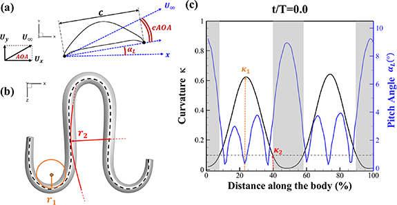
Figure 3. Definitions of (a) the angle of attack (AOA), the effective angle of attack (eAOA), the local pitching angle (), and the chord length (). (b) The snake curvature based on the inscribed circles. (c) The and curves are displayed as a function of body location, in black and blue lines, respectively. Two corresponding locations (large curvature) and (small curvature) are indicated in both (b) and (c).


Download figure:
Standard image High-resolution imageTo correlate the local pitching angle () to horizontal undulation, we use curvature to describe the horizontal shape of the snake, as shown in figure 3(b). The curvature at a point along the midline of the body is defined to be the reciprocal of the inscribed circle in the formula of:


The relation between and can be established as shown in figure 3(c), displayed in black and blue lines, respectively. The dashed black line indicates , and the region with curvature lower than 0.1 is highlighted in grey. The clear indication can be identified as the body parts with low curvatures possessing higher local pitching angles.


2.2. Computational methods and simulation setup
The governing equations solved in this work are the incompressible Navier–Stokes equations, written in an indicial form as
where are the velocity components, is the pressure, and is the Reynolds Number, which is defined as follows:


where denotes the kinematic viscosity of air. is the incoming flow at 20, and is the chord length of the snake cross-section shown in figure 3(a). In accordance with the previous study, the Reynolds number is set to 500 [10].


The governing equations are solved using a sharp-interface immersed-boundary-method-based in-house-developed flow solver with DNS, which allows for detailed fluid behavior around the thin edge features of the snake body [18]. A second-order Adams–Bashforth scheme is used for the convective terms, and the viscous term is solved using an implicit Crank–Nicolson scheme. This solver has been successfully applied to insect-inspired flapping or revolving wing propulsions [16, 19], hummingbird forward flights [20], and the aerial undulatory gliding of flying snakes [10, 21, 22].
The schematic of the computational domain is shown in figure 4(a). A domain size of 80c × 100c × 100c with an x–y–z coordinate system is set up, with a minimum grid spacing at = 0.164, as indicated in the dense dark blue region in figure 4(a). Utilizing a tree-topological local mesh refinement (TLMR) technique, the mesh around the flying snake model can be further refined with efficient computational resources [23]. From the enlarged schematic in figure 4(a), a larger parent mesh refinement block (light blue) encloses the wake region to resolve a semi-dense grid spacing at = 0.082c, and a smaller block (orange) around the snake model to capture the near-body vortices with a dense grid spacing at = 0.041c, resulting in a total grid count at 10.4 million. This mesh refinement technique has been applied to bio-inspired flight and animal swimming [10, 15]. An incoming flow velocity is applied in the x- and y-direction at an AOA of 35°, and a homogeneous Neumann boundary condition at the rest boundaries.


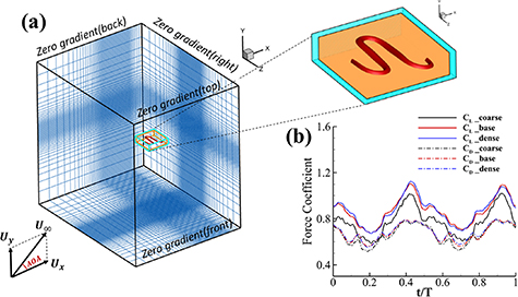
Figure 4. (a) Cartesian grid setup and nested topological local mesh refinement (TLMR) blocks with boundary conditions specified. The zoom-in figure shows the relativity of the blocks. (b) Mesh-independent study results with instantaneous and for a dense grid (Δ =0.035c, 13.98 million grids), a coarse grid (Δ = 0.082c, 3.02 million grids), and a base grid (Δ =0.041c, 10.39 million grids) used for the subsequent analyzes.


Download figure:
Standard image High-resolution imageThe grid-independent study was conducted using three grid sizes (for the orange inner block) at = 0.082c (coarse), = 0.041c (base), and = 0.035c (dense). The lift and drag coefficients, and , defined as the lift and drag forces and normalized by , are used to evaluate the mesh sizes. The force coefficients over a motion cycle are plotted in figure 4(b), where the solid line indicates and the dashed line indicates . The peak difference of and between the base grid and the dense grid is 1.8% and 0.05%, respectively, and the difference of the cycle averaged lift and drag coefficients between the base and the dense mesh is less than 0.1%. Therefore, we conclude that the base mesh is sufficient for the computation, and the analyzes herein are conducted with the base mesh.


2.3. Measurement of aerodynamic performance
The performance in the current study is evaluated through derived normalized variables. The lift (), drag (), and power consumption are non dimensionalized into coefficients of lift (), drag (), and power (), respectively, defined as


where and represent the instantaneous lift and drag force acting on the body, and they are defined as the forces perpendicular and parallel to the incoming flow. The undulatory power consumption is calculated as , where represents the surface integration of stress tensor and the velocity vector adjacent to the snake surface.


In gliding flights, the L/D is usually considered as one way to describe the gliding performance [5, 24]. It roughly represents the horizontal distance traveled at the cost of vertical drop in equilibrium gliding, thus evaluating the gliding efficiency. In this simulation, we compute the L/D with the ratio of the lift and drag coefficients:
Previous studies on insect hovering flights have discussed the lift-to-power ratio to evaluate the aerodynamic performance [25]. A similar definition of mean force-to-power ratio is adopted in this paper to define the cycle-averaged lift-to-power ratio () and the drag-to-power ratio () for additional performance evaluation metrics.


3. Results and discussions
This section presents the simulation results for the vertical-undulating model. Section 3.1 examines the aerodynamic performance of the baseline case and the vortex structures that lead to the performance. Section 3.2 compares the effect of different vertical wave undulation amplitudes () on the performance and flow features. Section 3.3 conducts the parametric study to investigate the effects of the dorsal–ventral bending () with varying amplitudes.


3.1. Baseline case
Figure 5(a) plots the instantaneous force coefficients of the baseline case from one steady undulating cycle. Clear symmetry in force productions can be observed as the vertical undulation motion is included, which is similar to our previous work on pure horizontal motion [10]. From figure 5(a), a peak lift production can be found at t/T = 0.41 in its right-to-left (R–L) stroke, rising from a global trough at t/T = 0.21. The drag generation history shares a similar trend to lift production, even though its trough and peak time is around 0.02 T ahead of the lift. In addition, it is worth mentioning that the change in drag production over a cycle is lower than that in lift production, implying the undulatory motion relates closely to lift production.
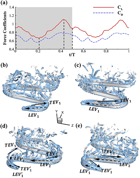
Figure 5. (a) The instantaneous force coefficients are displayed as the function of time in one undulatory cycle. The right-to-left (R–L) motion is shown in grey. 3D wake structures of flying snake model in the R–L stroke at (b) t/T = 0.00, (c) t/T = 0.21, (d) t/T = 0.41, and (e) t/T = 0.50 are presented in perspective view, respectively. The wake structures are visualized by the Q-criterion at values of 800 (in transparent white) and 1200 (in blue). The solid arrow indicates the directions of trailing-edge vortex tubes (TEV), and the dashed line arrow indicates the directions of leading-edge vortex tubes (LEV).
Download figure:
Standard image High-resolution imageThe instantaneous 3D wake structures of the flying snake in the R–L motion are visualized through the iso-surface of the Q-criterion [26]. Figures 5(b)–(e) plots these flow features at different time instants at t/T = 0.0, 0.21 (global minimum lift production), 0.41 (global peak lift production), and 0.50 to show the vortex development that corresponds to the force productions over the first half of a cycle as the motion in the following half-cycle is symmetric.
From figure 5(b), a pair of vortex tubes of LEV and trailing-edge vortex (TEV) (denoted as and ) can be identified near the leading edge and the trailing edge of the anterior body at the early stage of vortex generation at t/T = 0.0. While the TEV is detached and scattered, the LEV is a more intact vortical structure. The LEV is shown to be attached to the snake's head as it crosses through the incoming flow, and it is shed as it proceeds further into the motion cycle. An LEV detachment at the head portion can be observed in figure 5(c) at t/T = 0.21, resulting in a lower lift production compared to the previous time instant at t/T = 0.0 as shown in figure 5(a). As mentioned previously, the lift production rises from the trough as the gliding motion proceeds and peaks at t/T = 0.41, and the corresponding vortex topology is shown in figure 5(d). In figure 5(d), the previous pair of LEV1 and TEV1 from figure 5(b) are now denoted as LEV2 and TEV2, which are observed to shed from the body. At this time instant, a newly formed LEV denoted as LEV1', is attached to the anterior region, leading to the peak lift production at the moment. The vortex topology at t/T = 0.50 in figure 5(e) shows identical vortex topology to figure 5(b) at t/T = 0.0 due to the kinematic symmetry, and therefore same force production.


To investigate the flow behavior differences in the trough and peak lift production depicted in figure 5(a), the vortex strengths in t/T = 0.21 and t/T = 0.41 are studied. Vertical slice-cuts in XOY planes at three lateral locations with vorticity contours are presented in figure 6. The locations of the slice-cuts at z/c = −3, 0 and +3, and they are indicated in the schematics to the left of each slice cut in figure 6. At t/T = 0.21, which corresponds with figures 6(a1)–(a3), the LEV1 can be identified along the anterior body. The slice at z/c = −3 (figure 6(a1)) shows a small LEV1, whereas the slice-cut at z/c= 0 shows a developed LEV1 at the straight part of the body. The well-developed LEV1 is also found on the slice-cut at z/c = +3 located at the U-turn body part, while the TEV1 is smaller compared to that shown in figure 5(a2). At a later time frame at t/T = 0.41, the head made the U-turn and formed a new LEV denoted as LEV12 in figure 6(b1). Meanwhile, LEV1 that developed previously remains attached to the surface with high strength. While at locations of z/c = 0 and 3 (figures 6(b2) and (b3)), the LEV2 is observed to attach along the snake body. Compared to the vortex topologies in figure 6(a), figure 6(b) shows more LEV attachments throughout three different slice-cut locations along body segments, resulting in a higher lift production at this time instant which is reflected in figure 5(a).

Figure 6. The vortex contours at t/T = 0.21(a) and t/T = 0.41 (b). (1)–(3) corresponds to the slice-cut locations at z/c = −3, 0 and +3, respectively.
Download figure:
Standard image High-resolution imageThe overall vortex generation shares a similar pattern as in previous work by Gong et al [10]. However, the existence of vertical wave undulation brings a different pattern to the vortex. The introduction of vertical wave undulation brings changes to the local pitching angle, as shown in figure 3. When the vertical undulation is considered, the twisting on the straight body results in a forward pitching on the body that leads to a smaller eAOA compared to that from the pure horizontal undulation motion, and this reduction in eAOA weakens the LEV vortex formation and therefore reduces the lift production.
3.2. Effect of the vertical wave undulation
In this section, we will discuss how the amplitude of vertical wave undulation affects the aerodynamic performance and vortex structures of flying snakes during gliding.
3.2.1. Aerodynamic performance
In figure 7, the cycle-averaged aerodynamic performances are presented as a function of the vertical wave undulation amplitude . Figure 7(a) presents the general trend of cycle-average force performance change, including lift and drag coefficient ( and ). It was found that the cycle-average lift performance reaches a peak at with an 11.3% enhancement compared to our baseline case ). Compared with that from the pure horizontal case), the from this case is also 1.5% higher. As the increases, the shows a general trend of decreasing amplitudes beyond the point of . Meanwhile, a similar trend is observed for the production, yet the value is slightly decreased by 0.9% at compared to the case with as shown figure 7(a). The cycle-averaged power consumption shows a similar trend as that of the . At a vertical wave undulation amplitude of , the shows to be 0.7% higher than a pure horizontal case) and 8.7% higher than the baseline case (). This general trend that the force production and the power consumption synchronize with the lift production may contain implications for the flying snake gliding flights. When experiencing larger force on the body, the snake tends to consume more energy to maintain the same undulatory locomotion during gliding.


Figure 7. Cycle-averaged aerodynamic performance of the snake model with different vertical wave undulation amplitudes (). (a) Lift, drag and power coefficients; (b) lift-to-drag ratio, lift-to-power ratio, and drag-to-power ratio.

Download figure:
Standard image High-resolution imageFigure 7(b) shows efficiency ratios including the L/D, lift-to-power ratio , and drag-to-power ratio defined in section 2.3. It is found that while the lift performance reaches a peak at , the maximum L/D shows up at with an enhancement of 4.3% compared to the baseline case. Compared with the pure horizontal case), small increments can increase the performance by 1.5% for and 4.8% for L/D. When increases beyond 5°, the trend of the performance decreases at higher amplitudes. From figure 7(b), it is observed that has the same trend as L/D that reaches to peak value at , which is 1.2% higher than a pure horizontal case) and 2.8% higher than the baseline case (). On the contrary, follows the reverse trend as such that it reaches a minimum value at , which is 3.4% lower than a pure horizontal case). However, when the exceeds 10, the keeps descending. In general, the cycle-averaged aerodynamic performances will increase when vertical wave undulation amplitudes () are small (), but decrease when are large ().


In figure 8(a), the lift coefficient history of one steady undulating period with different is shown. Despite the similarity of force production trend, significant improvements can be found for the configuration of at t/T = 0.21 and 0.41. According to figure 8(a), the trough value of (t/T = 0.21) of is only 17.3% and 24.1% higher than that of and 20°, while the peak value of (t/T = 0.41) value of is 15.8% and 51.1% higher than that of and , respectively. The drastic difference in the peak value indicates that the near-body vortex structures will be the most different at t/T = 0.41, which will be discussed in the following.


Figure 8. Instantaneous aerodynamic performance of the snake model with different vertical wave undulation amplitudes at 2.5°, 10° (baseline case) and 20° over one undulatory cycle. (a) Lift coefficient, (b) drag coefficient, and (c) power coefficient. The two dashed lines are indicating the two time instants t/T = 0.21 and t/T = 0.41 for comparison.

Download figure:
Standard image High-resolution imageIn figures 8(b) and (c), the instantaneous drag and power coefficients over a cycle of motion are presented. The drag production and power consumptions are consistently higher for the case at over a motion cycle compared to those by the baseline case, while those at are lower. However, the reduction in power consumption is less than the loss in the lift production at , resulting in a lower cycle-averaged lift-to-power ratio as shown in figure 7(b). The instantaneous performance plots in figure 8 show the peak difference occurs at t/T = 0.41, and these performance differences are correlated to the flow phenomenon with detailed vortex dynamic analysis in sections 3.2.2 and 3.2.3.


3.2.2. Surface pressure and force distribution
Figure 9(a) shows the normalized local lift distribution along the body at the time instant at t/T = 0.41 to analyze the high and low force regions on the body, for the cases demonstrated in figure 8. The local lift coefficient is normalized with its overall lift , and the normalized lift coefficient indicates the variation of local lift force generation along the snake body. From the curve, we would observe that the 10%–20%, 45%–60%, and 80%–100% portions along the body tend to provide a similar amount of lift for different . The significant difference occurs between 20%–43% and 60%–83% regions indicated in grey. It is observed that the normalized peak value has been reduced by 200% ( () = 1.5 vs. () = 0.5). When is higher than , the lift production in these two regions is significantly reduced, which leads to the overall lift reduction.


Figure 9. (a) Normalized lift distribution along the body at t/T = 0.41 at different vertical wave undulation amplitudes at 2.5°, 10° (baseline case), and 20°. (b)–(d) Pressure difference contours () between ventral and dorsal surfaces of the snake body.


Download figure:
Standard image High-resolution imageTo further show the force distribution of the pressure force on the body, we define the pressure coefficient as:
Figures 9(b)–(d) present the corresponding contours of the pressure coefficient difference (), defined as , at different . It is observed that at , the straight parts of the snake body possess higher pressure difference of larger regions compared to the other configurations. The red zone of the lift generation becomes shallower as the increases while the force production near the curved portion of the body remains high. This lower at the straight body part corresponds to the lift loss region indicated in figure 9(a), which contributes to the decrease in the cycle-averaged lift production. Furthermore, the fact that the force difference occurs at the straight portion of the body indicates a different vortex strength across varied .


It is worth noting that the way in which a snake distributes its lift along the body suggests a possible strategy for controlling its movements while gliding. Although undulating in a way that causes large vertical waves may result in a loss of lift and reduced efficiency, it has been observed in nature that undulatory motion can involve large vertical deformations [11, 14]. The maximum we examined in this paper is at 20°, while in some occasions flying snakes in nature exhibit a higher at 30° [14]. From figures 9(b)–(d), the lift at the U-turn regions of the snake remains consistent regardless of the change. With increasing , more force will be concentrated on the lateral sides, the U-turn configurations of the body posture. The force concentration on the sides may imply a way snakes utilize to balance the force while gliding through the air.


3.2.3. Vortex dynamics and flow analysis
In this subsection, we will go into a detailed analysis of the effect of vertical wave undulation amplitudes. According to the previous discussion, we picked the key time instant t/T = 0.41, a time instant when the lift production reaches the peak, for detailed analysis and revealed the flow physics and flow change process for two different .

Figure 10 shows the instantaneous vortex structure at t/T = 0.41 with different of and , as well as the 2D span-wise vorticity () and fluid pressure coefficient () contours on the slice-cuts located at the XOY planes (whose locations are z/c = −3, 0, and +3, respectively). The vortex structure shows the same pattern as in figures 5 and 6. From the perspective view of the wake structure in figures 10(a1) and (b1), major vortex structures including the LEVs and the TEVs can be identified in the flying snake model. The maximum lift generation corresponds to the time instant when the longest LEV tube is formed and attached to the leading edge of the snake body. This feature holds when increases, implying the robustness of LEV-based lift generation in flying snakes gliding flights.


Figure 10. Flow information at t/T = 0.41 from different vertical wave undulation amplitudes at (a) 2.5° and (b) 20°. Near body 3D vortex topologies are plotted in (a1) and (b1). The corresponding 2D spanwise vorticity () and the fluid pressure coefficient () contours are plotted on the XOY slice-cuts located at (a2)–(b2) z/c = −3, at (a3)–(b3) z/c = 0, and at (a4)–(b4) z/c = +3.


Download figure:
Standard image High-resolution imageThe local span-wise vorticity and the corresponding fluid pressure coefficient contours are shown in figures 10(a2)–(a4) and (b2)–(b4), with clear connections between the vortex structures and the pressure zone identified. Figures 10(a2)–(b2) and (a4)–(b4) show the slice-cuts near the lateral sides of the U-turn body part of the snake. The 2D span-wise vorticity contours show that the generated keeps attached to the leading edge of the body, which corresponds to higher force productions at these regions as shown in figure 9. Specifically, the structures show evenly distributed strengths along different body portions, and the corresponding low-pressure zones on the dorsal side are of similar strengths as shown in figure 10(a2). However, although the vortex structures remain similar with a higher vertical bending amplitude at , the dorsal side low-pressure zones at the posterior body part are of lower strengths as shown in figure 10(b2), resulting in the posterior lift reduction in figure 9(a). As for the U-turn section on the other side of the body, the formed on the trailing edge is closely attached to the dorsal surface of the body for shown in figure 10(a4). The low-pressure zones induced by the and are mutually enhanced with close attachments to the dorsal side of the body at the U-turn section, allowing for low surface pressure regions at the U-turn body part. With higher vertical undulation amplitude at shown in figure 10(b4), the on the upstream body part is more scattered, while is convected further downstream that results in the decreased strength of the low-pressure zone with less lift generation. This is consistent with pressure difference contours shown in figures 9(b) and (d), as the lift generation in the U-turn section is lower on compared to that on .


The midplane slice-cuts are presented in figures 10(a3) and (b3). Due to the large vertical undulation amplitude, the cross-section of the snake experiences a large local pitching angle forward. Based on the previous study by Gong et al [10], at smaller pitching angles (<), the lift production will decrease with the AOA. Here, in the mid part of the body, where the snake has a small curvature and straight body, the reduction of eAOA causes the weaker vortex formation. In figure 10(a3), the remains attached to the body, while in figure 10(b3) the is detached from the leading edge resulting in lower lift productions. The corresponding pressure contours in figures 10(a3) and (b3) also indicate the vortex strengths formed in the gliding configuration of to be weaker, as the low-pressure zones induced by the vortices are of reduced strengths compared to those from . This lift-related vortex formation is highly related to the eAOA. For , the eAOA near the straight portion of the body is optimal, bringing an overall maximum lift production as shown in figure 7(a). On the other hand, the eAOA on the body with is reduced with a lift loss on the straight body portion. Compared to the middle section with relatively straight body parts, the lateral sides in figures 10(a2) and (a4) are less affected by the local eAOA due to the body U-shape turning. This implies that in gliding flights, the snake tends to minimize the local pitch angle in order to maintain a smooth body.


3.3. Effect of the dorsal-ventral bending
As stated previously, flying snakes also apply the dorsal–ventral bending motion in addition to the vertical bending motion as an alternative way to achieve vertical deformation. Without a sinusoidal wave, the dorsal–ventral bending describes a gradual linear transition from the head to the tail as indicated in figure 2. This motion is often observed as the snake maintains its head steady while its tail bends upwards or curls downwards. As described in equation (2), is the dorsal–ventral bending amplitude that we used to investigate the effect. indicates a tail-down configuration, and indicates a tail-up configuration. This section serves to explore the effect of on the aerodynamic performance with the optimal found previously.


3.3.1. Aerodynamic performance
Figure 11 presents the change in cycle-averaged aerodynamic performances with varied dorsal–ventral bending amplitudes . In figure 11(a), the cycle-averaged lift, drag, and power coefficients follow a monotonically increasing trend with from to . At , the overall lift production increases up to 1.02, equivalent to a 17.3% cycle-averaged lift enhancement compared that from the baseline case, and this enhancement is even higher than that from the optimal case at , when we only consider the vertical wave undulation amplitude . This means the snake tends to generate higher lift more efficiently when its tail bends downward. When increasing the dorsal–ventral bending amplitude to generate more lift, the flying snake consumes more power to maintain the undulation motion during the gliding flying, and consequently higher aerodynamic forces ( and ) are produced.


Figure 11. Cycle-averaged aerodynamic performance of the snake model with different dorsal-ventral bending amplitudes (. (a) Lift, drag and power coefficients; (b) lift-to-drag ratio, lift-to-power ratio and drag-to-power ratio.

Download figure:
Standard image High-resolution imageFigure 11(b) describes the and as monotonically decreasing with the increase of while is less affected, and the variance among different data is less than 1.0%. This indicates that compared to the tail-down motion, the tail-up motion is a more efficient posture during gliding, allowing for lower drag production and power consumption. Compared with the baseline case (), at , L/D = 1.35 and it is 5.8% higher. also shows a 4.5% enhancement as we decrease to . However, the lift production is reduced by 15.6% simultaneously due to less overall force production.


To understand the instantaneous performance change from the dorsal–ventral bending angle , the instantaneous performances over a cycle are shown in figure 12 with different dorsal–ventral bending amplitudes. Unlike the change with where significant difference only appears at some time periods, such as t/T = 0.21 and t/T = 0.41 indicated in figure 8, the performance changes from the dorsal–ventral bending is consistent throughout a motion cycle. This means that the effects of the dorsal–ventral bending on the aerodynamic performance of the flying snake are not limited to certain parts of the body, but altering force productions along its body instead.


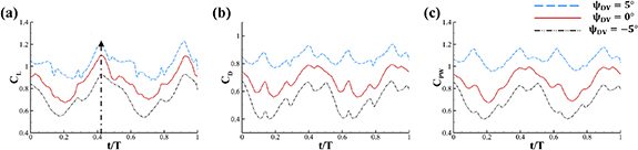
Figure 12. Instantaneous aerodynamic performance of the snake model with different dorsal-ventral bending amplitudes at 5°, 0° (baseline), and −5° over one undulatory cycle. (a) Lift coefficients, (b) drag coefficients, and (c) power coefficient.

Download figure:
Standard image High-resolution image3.3.2. Vortex dynamics and flow analysis
The instantaneous 3D vortex structures for cases with at and are shown in figure 13 at the same time instant as in the previous analysis at t/T = 0.41, alongside the 2D span-wise vorticity () and fluid pressure coefficient () contours on the slice-cuts in a same style to figure 10. The general vortex structures appear similar to the baseline case as shown in figure 5, despite a difference in the distance between the vortex tubes and the body surface due to the ascending or descending body postures. Figure 13 (a1) shows the vortex structure for the tail-up case (), and figure 13(b1) shows that for the tail-down case (). For the tail-up case, the LEV and TEV tubes appear to be closer to the surface of the body, which will result in a stronger effect on the body force. On the other hand, the tail-down case shows a more complex vortex structure that may connect to the enhanced aerodynamic performance.


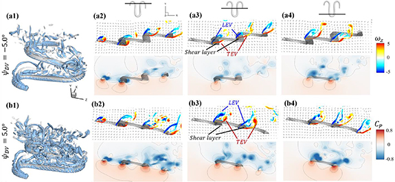
Figure 13. Flow information at t/T = 0.41 from different dorsal–ventral bending amplitudes at (a) −5.0° and (b) 5.0°. Near body 3D vortex topologies are plotted in (a1) and (b1). The corresponding 2D spanwise vorticity () and the fluid pressure coefficient () contours are plotted on the XOY slice-cuts located at (a2)–(b2) z/c = −3, at (a3)–(b3) z/c = 0, and at (a4)–(b4) z/c = +3.


Download figure:
Standard image High-resolution imageIn the same style as the slice-cuts in figure 10, the vorticity contours and the pressure coefficient contours are plotted in figure 13 for both the tail-up and the tail-down configurations. The flow pattern affected by the dorsal–ventral bending angle correlates with the overall performance changes observed in figure 12. For the tail-up configuration () shown in figures 13(a2)–(a4), the body posture inclination generally aligns with the flow direction, according to figure 3(a). This positions the posterior body parts of the snake model within the wake produced by the anterior body parts. To start, we will analyze the vortex formations that occur around the U-turn sections. As shown in figure 13(a2), the posterior body part is positioned immediately downstream from the upstream wake, causing the vortices shed by the upstream U-turn section to affect the vortex formations on the downstream U-turn section directly. Similar changes in posterior body performance due to wake effects were observed in the 2D study of foil–foil interactions by Jafari et al [12]. However, the interaction between the fore and aft sections is diminished for the other side, as shown in figure 13(a4), due to the presence of one U-turn section. In the tail-down configuration ) shown in figures 13(b2)–(b4), the posterior body part is positioned away from the wake region of the anterior body. As the distance increases, the interaction between the wake and body diminishes. Consequently, vortex formation on the posterior body part of the body in the tail-down configuration is less affected. This section experiences flow conditions that are less disturbed by the upstream body parts. This leads to uniform distributions of ventral high-pressure zones for all body parts, as shown in figures 13(b2) and (b4). When comparing the fluid pressure contours on the posterior body part of the snake's body in the tail-up and tail-down configurations, the pressure gradient across the top and bottom surfaces of the snake body is consistently weaker in the tail-up configuration than in the tail-down configuration.


Figures 13(a3) and (b3) compare the vorticity and the fluid pressure contours on the slice-cut at the middle of the straight body part with different . At , the LEV structure on the posterior body has a smaller scale compared to that on the posterior body at . This can be explained by examining the velocity vector field, as the flow immediately ahead of the posterior body part is strongly affected by the presence of the TEV on the anterior body in figure 13(a3), resulting in diminished LEV circulation strength on the posterior body. Moreover, the eAOA on the straight middle body part is higher in the tail-down configuration than in the tail-up configuration, and therefore stronger LEV structures as shown in figure 13(b3). Therefore, by changing the in the gliding motion, it changes the vertical distance between the anterior and the posterior body parts that dominate the wake-body interaction effectiveness, and it also changes the eAOA on the straight body part that is responsible for the lift-producing LEV generation.


Tucker and Conlisk [27] provided the vortex-wedge interaction profiles where in their physical model, the triangular wedge collides with the upstream wake and vortices. By shifting the distances between the body and the wake, they found out that the vortex breakdown switches from above the top surface to the leading edge. As a result, the LEV and TEV distort and merge with the shear layer on the bottom surface. Here in our current research, we also noticed that the distance between the snake body and the wake affects the aerodynamic performance accordingly. Similar trends of location shift along with vortex breakdown have been summarized in [28, 29]. The effects of the upstream body wake on the downstream parts have also been studied in other bio-inspired flows such as fish swimming in dynamic wakes. When the fish is located in the vortex flow induced by an upstream body, it may exploit the incoming vortices resulting in drag reduction and preferable energy expenditures [30, 31], which is consistent with the interaction present in the current study.
Figure 14 plots the contours for the cycle-averaged local U-velocity change () and for the cycle-averaged fluid pressure coefficient (), at the midplane slice-cut in the flow for different . In figure 14(a), the blue color is defined as negative U-velocity, which represents a reversed flow in the wake. In the downstream wake, the flow speed is usually smaller than that of the incoming flow due to the flow separation and interaction, similar to the flow features in the von Karman vortex street. In figure 14(a1), the two wakes merge into one in the tail-up configuration, while a distinct two-wake street pattern is shown in the baseline case as shown in figure 14(a2). Differences between the tail-up configuration and the baseline case mainly come from the posterior body wake, while similarities are found in the wake of the anterior body part by comparing figures 14(a1) and (a2). The posterior body wake is also significantly reduced by merging into that from the anterior body. The two-street wake pattern in the baseline case is more distinctive with higher at . Consistent with our previous analysis, the has a more significant impact on the posterior body, due to the merger of LEV and the counteract of TEV as shown in figure 13. From figure 14(b1), it is also observed that there is only one high-pressure region below the body in the anterior body part, compared to that from the baseline case in figure 14(b2) showing a secondary high-pressure region near the middle body part. Furthermore, the low-pressure region in the top side of the snake model is of lower strength in the tail-up configuration compared to the baseline case. As previously analyzed, decreasing pressure difference brings less lift component, especially for the posterior body. On the other hand, the force component aligning with the flow direction decreases as well, resulting in lower body drag production to realize the overall preferred L/D.


Figure 14. Cycle averaged (a) local velocity contour and (b) pressure contour with different dorsal-ventral bending amplitudes of (1) −5.0°, (2) 0°, and (3) 5.0°. The location of the XOY slice-cuts is at z/c = 0. Dashed lines indicate the wake region. Black arrows indicate the force direction caused by the pressure difference.

Download figure:
Standard image High-resolution imageAs for the tail-down configuration (), the distance between the wake drifted apart due to the dorsal–ventral bending downwards in figures 14(a3) and (b3). Contrary to the reduced wake width from the posterior body shown in figure 14(a1), the tail-down configuration shows an increased wake width for the posterior body part. Compared with the baseline and tail-up () cases, the tail-down configuration possesses enhanced low-pressure regions in the top surface as shown in figure 14(b3). The high-pressure regions below the body is also enhanced, resulting in an additional high-pressure region at the tail part of the body. This cycle-averaged high-pressure difference brings higher lift production to the overall body, which agrees with the overall increasing lift trend presented in figure 11(a). At the same time, the drag force production is also increased alongside the gliding power consumption, which reduces the lift-to-drag and the lift-to-power ratio during the flying snake's aerial gliding.


4. Conclusions
In this study, the effects of vertical bending locomotion on the aerodynamic performance in flying snake's gliding flights are investigated numerically using a 3D snake model featuring a realistic snake-like cross-sectional profile and equation-controlled undulation kinematics. Herein, we focused on the investigation of the two most influential parameters in the vertical bending motion that would lead to significant performance change, including the vertical wave undulation amplitude and the dorsal–ventral bending amplitude .


Our findings show that horizontal undulation plays a key role in vortex formation. We consistently observed the formation of oblique LEVs and TEVs across various vertical bending configurations. Notably, maximum lift generation occurs when both LEVs are attached to the straight parts of the S-shaped body posture. This suggests that the lift-producing mechanism related to LEVs, identified in our previous study [10], is consistent in the gliding flights of flying snakes.
Results show that the vertical wave undulation amplitude () enhances aerodynamic performance when the amplitude is small, while its further increase deters the lift production. For a small increment compared with pure horizontal undulation, the force production increases and reaches a peak at = , while the L/D and reach a peak at = . When further increases, both the lift production and the efficiency decrease. The reduction in high amplitude of vertical wave undulation is identified to be the reduction in the local eAOA, especially for the straight portion of the body that results in lift loss.


Dorsal–ventral bending (), an important vertical motion, contributes to the aerodynamic performance through a different mechanism. As increases, the tail curls downward and separates the distances between the bodies and the anterior body wake. As the distance between the upstream and downstream body parts increases, the interaction between the wake and the body weakens. The posterior body produces significantly higher lift when the snake bends downward away from the wake, at the cost of slightly increased power consumption, resulting in a lower ratio in the tail-down motion. Conversely, decreasing the angle bends the snake tail upward, leading to different aerodynamic performance. The locations of the posterior body parts being in the wake of the anterior body increase the interaction between the wake and the body, which reduces force production and power consumption. This results in improved gliding efficiency.


By adopting different dorsal–ventral bending, the flying snake can adjust its gliding strategy to gain more lift for deceleration or achieve more efficient gliding. This trade-off in aerodynamic performance, achieved by simply altering its body posture, indicates flying snakes may use active body control during gliding flight to achieve high maneuverability. These findings are expected to deepen our previous knowledge of flying snake gliding and to inspire the design of agile gliding snake-like aerial robots.
Acknowledgment
This work is supported by NSF Grant CBET-2027534. The UVA Research Computing Group provided Computational resources on the UVA Rivanna computing cluster.
Data availability statement
The data cannot be made publicly available upon publication because they are not available in a format that is sufficiently accessible or reusable by other researchers. The data that support the findings of this study are available upon reasonable request from the authors.