
Abstract
During walking, sensory information is measured and monitored by sensory organs that can be found on and within various limb segments. Strain can be monitored by insect load sensors, campaniform sensilla (CS), which have components embedded within the exoskeleton. CS vary in eccentricity, size, and orientation, which can affect their sensitivity to specific strains. Directly investigating the mechanical interfaces that these sensors utilize to encode changes in load bears various obstacles, such as modeling of viscoelastic properties. To circumvent the difficulties of modeling and performing biological experiments in small insects, we developed 3-dimensional printed resin models based on high-resolution imaging of CS. Through the utilization of strain gauges and a motorized tensile tester, physiologically plausible strain can be mimicked while investigating the compression and tension forces that CS experience; here, this was performed for a field of femoral CS in Drosophila melanogaster. Different loading scenarios differentially affected CS compression and the likely neuronal activity of these sensors and elucidate population coding of stresses acting on the cuticle.
Export citation and abstract BibTeX RIS

Original content from this work may be used under the terms of the Creative Commons Attribution 4.0 license. Any further distribution of this work must maintain attribution to the author(s) and the title of the work, journal citation and DOI.
1. Introduction
Locomotor coordination requires the integration of sensory information to modify or reinforce motor patterns while organisms adapt to dynamic environments. Sensory information is measured and monitored by sensory organs that can be found on and within various limb segments. Mechanosensory neurons on limbs, such as the legs, can provide highly specific information on limb position and movement—created by muscles and the neuromuscular system as well as those by the environment acting on the body—which, in turn, can modify the intrinsic network output controlling the movement of each leg [1–6].
For decades, continuing advances in research into the neurobiology of motor control and a biology-first approach to robotics have complemented each other [7]. This research has highlighted the benefits of utilizing sensory feedback systems for limb coordination as well as the robust benefits of using biomimicry in robotics. However, understanding mechanosensory feedback in insects to the degree necessary for robotic implementation has been strenuous due to the involvement of both neural and mechanical properties [1, 8]. Computational and physical models can aid in the investigation of all factors contributing to the versatility and flexibility in insect and arachnid walking [9–15]. Ultimately, walking robots can be equipped with bio-inspired sensors that reduce computational costs while increasing, for example, the speed of recovery from perturbations [16].
Interdisciplinary collaboration in the form of physical, robotic modeling of animals facilitates research into highly complex phenomena influencing motor control. For example, when a leg cycles between its stance and swing phase, the accompanying forces change over time [17, 18]. These forces, in turn, create varying directional stresses within the exoskeleton, which can lead to physical deformations. These strains are encoded by dynamic force sensors in insects, called campaniform sensilla (CS) [10, 19–21]. Due to the interplay of dynamic stresses and strains and the corresponding adaptive neuronal activity, CS mechanics and responses are highly complex, requiring interdisciplinary approaches to understand the mechanisms underlying their function (figure 1). Recent work integrating CS-like strain sensors in robotic legs modeled off of stick insect legs [22, 23] demonstrated how the application of appropriate forces could evoke strain patterns similar to those measured in the insect leg itself [24]. Further work [23] showed how these artificial limbs could be used to answer questions that, to date, could not be answered using real animals, such as how species-specific CS locations determine the components of leg strain they can detect. This is mainly possible due to the fact that CS are sensitive to changes in force, which can be modulated by body weight [25], substrate movement [20], and naturally occurring bending moments during stepping [26].

Figure 1. Schematics detailing the femoral CS field, directional sensitivity and range fractionation, CS morphology, and model implementation; (A) detailed image of a wing-less Drosophila with red dot marking the approximate location of the femoral CS field on the middle leg; coordination cross shows the movements of the femur; (Ai) schematic of a Drosophila leg; red dot marks the approximate location of the femoral CS field; arrows show the movement of the distal femur during, for example, resisted muscle force, this would lead to compression on the dorsal side of the femur and tension on the ventral side of the femur; Adapted with permission from [27]. © 2020 The Authors. The Journal of Comparative Neurology published by Wiley Periodicals LLC. CC BY-NC 4.0; (B) schematics of a circular and elliptical CS; there are no shorter axes in the circular CS, thus all forces from any direction can lead to compression along all axes; in elliptical CS the shorter axes is more sensitive towards compression then the longer axes; this leads to directional sensitivity through the orientation of the ellipse; (Bi) schematic showing the effects of range fractionation; the smaller the ellipse the less force is needed to lead to short axes compression; (C) schematic of a simplified CS setup based off of Grünert and Gnatzy [28], Moran et al [29], and Dinges et al [30]; L, layer; (C1) image of the 3D resin-printed model made out of three different resins; arrows indicate which aspects of the CS schematic are replicated.
Download figure:
Standard image High-resolution imageIn addition to location and orientation, CS transduction and activity depend on their material and cellular properties (table 1). Each CS consists of one mechanosensitive neuron with a modified dendrite that interacts with CS components that are embedded within the exoskeleton [10, 21, 29, 31]. The exoskeletal components include a cap, a dome-shaped structure that can vary in eccentricity [29, 31–33], which is sometimes surrounded by a collar, a ring like structure that connects the cap to the surrounding cuticle via a joint membrane [28, 34]. The joint membrane may function as a gap filler [35]. The cap is thought to consist of two layers, one of these consists of relatively stiff, tanned cuticle [35] and the other has material properties similar to those of resilin [29, 34, 36, 37]. As resilin is rubber-like and very elastic, it has been postulated that this layer allows CS to resume their resting configuration after displacement [34, 36, 38, 39]. Below these structures, and surrounding the modified dendrite, are sockets, also known as socket septa [28, 40]. These sockets may be involved in stimulus transmission and they differ from the collar and cap in their elastic properties, which affect strain amplification [8, 35, 40, 41].
Table 1. CS attributes and their potential effects on strain sensing
| Attribute | Effect | Mentioned in: |
|---|---|---|
| Cap: | ||
| Shape & eccentricity | Low eccentricity CS are more omnidirectionally sensitive, while high eccentricity caps are directionally sensitive; can also effect the sensory neuron morphology | [22, 24, 25, 34, 35, 37–41 et al] |
| Orientation | Determines CS sensitivity; limits responsiveness | [24, 25, 34–37 et al] |
| Size | Determines the necessary force for sufficient cap displacement; can contribute to range fractionation or filtering for signal fractionation | [33 et al] |
| Sockets/socket septum | Interconnected sockets affect strain propagation within a field; limit extent of displacement | [42, 43 et al] |
| Collars | May tune sensor sensitivity; possible protective function; can alter omnidirectional responsivity of more circular CS, can affect global strain | [30–33, 39 et al] |
| Grouping of multiple CS | May allow range fractionation and encoding of stress arising from different directions, allows greater sensitivity than a single CS, compensate for loss of sensors, noise reduction, can amplify strain | [31, 44–47 et al] |
| Material properties | Affect amplification of strain; alters sensitivity; cap compliances can act as a filter | [28, 30, 42, 48 et al] |
| Placement/position on limb | Inconsistencies in cuticle can effect strain distribution; mechanical hysteresis can stiffen caps; viscoelasticity can affect the CSs' tuning to the rate of change in strain over time, local geometry affects CS; affects strain magnitude | [25, 28, 31, 32, 44, 49–51 et al] |
CS are found as individual sensors or in groups throughout the leg, with larger collections generally in more proximal leg segments. CS can be clustered into groups or fields, with differences in CS cap size, eccentricity, and orientation within these areas. Variations in cap size allows range fractionation, in which the strain magnitude is encoded within the limited sensitivity ranges of each individual cap, with the activity of the entire field encoding a broad range of strains [52, 53]. Once a response-evoking strain reaches a cap, the cap displaces laterally through compression forces [29–31, 34–36]. This movement can activate mechanosensitive ion channels in the CS neuron's modified dendrite [31, 36, 54], ultimately allowing the cuticular strain to be encoded with nanometer-scale sensitivity [41, 55, 56]. Differences in cap eccentricity create directional or omnidirectional sensitivity in CS [46, 47, 57]. Caps with eccentricity closer to 1 are most sensitive to compression along their shorter axis, creating directional sensitivity according to the orientation of this axis relative to those of the limb segments [43, 44, 46, 48, 51, 58, 59]. Caps with eccentricities closer to 0 have omnidirectional sensitivity, as all axes should compress similarly [57], although the presence of a collar can modify this omnidirectionality [47]. All of these aspects influence the neuronal encoding and signaling of strain. However, methodological limitations, such as the size of the limbs and strain magnitude, as well as missing driver lines for efficient neuronal activity monitoring in Drosophila, make it difficult to connect this strain to neuronal function in groups of CS.
We used a physical model of the femoral CS field of D. melanogaster due to the varying CS morphologies within this location and the assumptions that have been made about its activity during walking (table 1). The resisted forces of the depressor muscle, which presses the leg and, thus, the femur against the ground during walking and jumping, should lead to dorsal bending of the femur, which should place the area of the femoral CS field (proximal ventral femur) under tension (figure 1(Ai)). Recent finite element analysis (FEA) of the femoral field also concluded that tensile displacement of the field could displace caps, with a predominant effect on more distal CS [30]. In addition, this field includes 8 elliptical CS, which should be directionally sensitive to torques because of the orientations of their long axes [44], as well as three circular CS, which should undergo strain amplification through their less-compliant collars [30, 35]. Finally, this field also contains caps with different sizes, which should create range fractionation during strain sensing [53].
Various studies, as early as in 1937 [10], have shown how strain can affect the function of CS throughout the insect body, as they are found on legs, wings, halteres, and antennae [31]. Vincent et al [60] modeled a CS field as holes in a plate, showing that a regular pattern of the holes in the surface could increase strain sensitivity, with even spacing leading to strain amplification. A study by Kaliyamoorthy et al [14] combined FEA and confocal microscopy to model the alternating strains that arise in the trochanter limb segment during climbing. A study by Dinges et al [30] also used FEA in combination with nano-computed tomography (CT) to investigate how physiologically correct strain affects cap displacement in one field while altering the elasticity of the collar and sockets. Further, Sun et al [54], investigated the displacement of haltere (a gyroscopic limb in Dipterans) CS while applying physiological forces and high-resolution imaging in combination with FEA.
Although these studies have been crucial for the field, using methods such as FEA commonly requires approximating some physiological aspects of the exoskeleton–neuron interface such as the composition of the cuticle—which affects CS firing [61]—and demand high computational capacity. In order to circumvent the difficulties of modeling viscoelasticity, as well as to implement models that can mimic the variability seen in the relative arrangements of CS within groups and fields [30], we developed a physical CS model based on nano-CT segmentation equipped with strain gauge rosettes to monitor strain under conditions closely mimicking the physiological state.
Many robots and robotic limbs use incorporated strain gauges for strain sensing, often mimicking leg CS or insect sensing [22, 23, 62–66], together with models of sensory neuron firing [19]. These systems are capable of predicting cellular activity by processing changes in resistance caused by strain in a fashion similar to animal experiments. Commonly, these robotic structures are built using additive manufacturing (3D printing), allowing the use of bioinspired or insect-first structures to reflect the physical diversity found in various insect species [67]. In the present study, we adopted an additive manufactured model consisting of cuticle and CS structures created using resins to incorporate various viscoelastic properties. Thus, this approach aimed to highlight the mechanistic function of CS as well as to establish a platform to test the effects of CS variability, integrating high-resolution imaging, and tensile testing with different loading forces and moments to identify the relationships between structure, location, and orientation in the context of sensory encoding and locomotion.
This investigation on the interplay between morphology and strain sensing demonstrated that (1) the utilization of resin printing was appropriate for capturing viscoelastic properties, (2) different loading forces and moments affected strain in a single CS field, (3) force could not only compress an individual cap but also skew or shear it, and (4) additive manufacturing is likely a useful resource to investigate insect biomechanics. This study advanced our understanding of proprioceptive strain sensory organs by outlining how cuticular structures filter and modulate mechanosensory inputs.
2. Materials and methods
2.1. Nano-CT and models
The nano-CT data from the femoral CS field of the fruit fly Drosophila melanogaster used to create our model were adopted from a previous publication [30]. This field has 11 CS with varying degrees of eccentricity and both collared and uncollared caps, making it an interesting model with which to study the effect of these features on load measurement. Using Blender rendering software (v3.2.1; Blender Foundation, Amsterdam, Netherlands) the segmentation mesh was remeshed (voxel size, 0.1; adaptivity, 9 m [object space]; smooth shading; remove disconnect) and the corrective smooth modifier (factor, 0.8; iterations, 15; scaling factor, 1.00) was applied to reduce mesh complexity for 3D printing (figures 2(A)–(Aiii)). The segmented caps were removed, and cylinders with the same dimensions were inserted as a substitution. These had a flatter surface towards the outside of the model and were slightly concave to the inside of the model. This was necessary for the application of the strain gauges. Collars are naturally found around three of the femoral field CS; these were also removed and substituted with rings with the same dimensions as the original collars. These were added to the model using the Boolean modifier in Blender. T-beam like structures were added to both the distal and proximal ends of the model using the Boolean modifier. This was necessary to connect the 3D printed model (figures 2(B)–(Biii)) to milled steel mounts (figures 2(C)–(Cii)) that connected the model to the tensile tester. The dimensions of each cap and collar and of the complete model are listed in table 2.

Figure 2. Model and its viscoelastic parameters; (A) remeshed and modified nano-computed tomography segmented model of Drosophila femoral CS field; caps (11) are represented in different colors; collars (3) are shown in white; T-bar-like attachments were added to the proximal and distal ends as attachment sites; (Ai) interior view of model; (Aii) right side of model; (Aiii) left side of model; (B) resin-printed physical model, exterior view; black arrows indicate collars (in white); caps are clear; cuticle is dark grey; different colors result from different resins; (Bi) interior view of model; (Bii) right side of model; (Biii) left side of model; (C) steel attachment for attaching the model to the tensile tester frame kit; the five tapped through-holes show different loading scenarios: centric, left, right, back, front; (Ci) interior view of (C); (Cii) side view of (C); (D) schematic of elliptical and circular CS, each with three axes; elliptical CS had short, long, and 45° axes; circular CS had BLTR (bottom left, top right), BRTL (bottom right, top left), and the corresponding 45° axes; blue, red, and green labeling depicts strain gauge axes aligned with CS axes; (E) schematic of experimental procedure with change in tensile tester velocity (rpm) shown in orange, consequent change in position magnitude shown in blue, and monitored force (N) in black; (F) force against microstrain measurements of short axis for all 11 CS.
Download figure:
Standard image High-resolution imageTable 2. Model dimensions [mm]
| Short axes/BLTR | Long axes/BRTL | Thickness | Width/length ratio | |
|---|---|---|---|---|
| Entire model | 50.46 | 77.52 | 2.02–3.12 | |
| Caps | Collar thickness | |||
| CS 1 | 4.22 | 4.97 | 1.07 | 0.84 |
| CS 2 | 3.82 | 5.80 | 0.65 | |
| CS 3 | 3.12 | 5.13 | 0.60 | |
| CS 4 | 6.54 | 5.97 | 1.25 | 0.93 |
| CS 5 | 6.34 | 6.58 | 1.34 | 0.96 |
| CS 6 | 4.73 | 6.78 | 0.69 | |
| CS 7 | 3.62 | 4.91 | 0.73 | |
| CS 8 | 6.26 | 8.51 | 0.73 | |
| CS 9 | 5.68 | 8.14 | 0.69 | |
| CS 10 | 4.41 | 7.14 | 0.61 | |
| CS 11 | 3.79 | 5.27 | 0.71 | |
| Strain gauge | 2.31 | 3.76 |
All measurements were completed using calipers on the physical model; CS, campaniform sensilla; BLTR, bottom left top right; BRTL, bottom right top left
2.2. Resin printing
The physical model (figures 2(B)–(Biii)) was printed using a Formlabs Resin Printer (Somerville, MA, USA). The caps were printed using Formlabs Elastic Resin (Elastic 50 A) with an ultimate tensile strength of 3.23 MPa [68]. The collars were printed using Formlabs Rigid Resin (Rigid 4000) with a Young's modulus of 4.1 GPa [69]. The cuticle was printed using Formlabs Tough 1500 Resin, with a post curing Young's modulus of 1.5 GPa [70]. The cuticle and collar resins were chosen based on the Young's moduli estimated for Calliphora vicina (cuticular cap, 6 GPa; collar, 4.8 GPa; cuticle, 1.5 GPa) [35]. The cap resin was based on a study showing that the cap consists of two layers, one of which is similar to resilin [29, 34, 36]. This layer is assumed to be connected with the collar, and may thus mechanically amplify strain onto the modified dendrite, which inserts directly into the cap [71, 72]. Resilin has a tensile strength of 4 MPa [73], and our model used Formlabs Elastic 50 A Resin (3.23 MPa). After printing, the caps and collars were manually mounted into holes in the resin cuticle structure. To solidify the connections, a thin layer of Elastic 50 A resin was cured to the inside of the model. Controls were completed using a square with T-bar ends made out of Formlabs Tough 1500 Resin (figure S1). The model was 2.36 mm thick, 77.28 mm in length, and 50.24 mm in width. One control consisted of only Formlabs Tough 1500 Resin, and the second control had a single circular inlet filled with a cylinder (6.81 mm × 6.81 mm × 2.36 mm) made out of Formlabs Elastic 50 A Resin in the center of the square.
2.3. Strain gauges and electronics
Strain gauge rosettes (Micro-Measurements C5K-06-S5198-350-33 F; Vishay Intertechnology, Toronto, ON, Canada; Grid resistance, 350.0 Ω ± 0.5%) were glued on to the caps using a thin layer of instant glue (schematized in figure 2(D)). These gauges included three measurement axes (0°, 45°, 90°). They were manually aligned with the corresponding short and long axes of the caps, and also measured the strain along the axis at 45° between the other two. Less eccentric caps (CS 1, 4, and 5) do not have long or short axes; for these, the strain gauges were oriented so that one axes was on the axis running from the bottom right to the top left (BRTL) of the circle and the other axis mirroring this BLTR. This was necessary because these "circular" CS, as to which they are often referred, are not perfectly circular [30]. Each strain gauge was amplified using a Wheatstone bridge in the quarter-bridge configuration, whose output was amplified by an inverted operational amplifier circuit. During displacement, the strain gauges underwent a change in resistance, producing an analog voltage signal at the amplifier output that was proportional to the sensor strain [22]. Signals were recorded by an Arduino Mega 2560 (Arduino, Turin, Italy) microcontroller with a Mux Shield 2 (Mayhew Labs, Carmel, IN, USA) multiplexer, which transformed the analog signals into a 12-bit digital signal. Readings were sent to a computer via serial connection and read in Arudino IDE software (version 1.8.15; Arduino).
In parallel, we used a manual hand wheel-operated test stand (FGS-250 W; Nidec-Shimpo Corp., Kyoto, Japan) equipped with a digital force gauge (1000 N ± 0.3% full scale accuracy; FG-3009; Nidec-Shimpo Corp.). The force measurements were read using EDMS force gauge software (v4.6.0; Nidec-Shimpo Corp.). The hand wheel included a tensile frame kit (FGS-250 W-TFK; Nidec-Shimpo Corp.). To connect the model with this frame kit, we crafted steel attachments into which the resin model could slide (figures 2(C)–(Cii)). These attachments had five tapped through-holes, into which the frame kit could be screwed. These different holes created different loading conditions for the model (centric, right, left, front, back). Right loading corresponds to anterior directed strains; left loading corresponds to posterior directed strains; centric loading is dorsally-directed force at the distal end of the femur; the back loading represents the same force, but with an extra force pulling into the body, like a muscle attachment; and the front loading represents the same distal femur force, but with a pressure pushing out of the body. These are approximate relations. We tested these conditions under tensile loading, as this should correspond to the force this field would experience when the animal walks or jumps from an upright posture (figure 1(Ai)). We also tested the centric condition under compressive force as a control. We replaced the tensile tester's hand wheel with a Dynamixel servomotor (XM540-W270; ROBOTIS Co., Ltd, Seoul, Republic of Korea) in order to produce constant motion and repeatable displacement parameters. The motor was controlled by Dynamixel Wizard 2.0 software (v2.0.16.4; Robotis Co., Ltd.). The motor speed was set at a velocity of 0.458 and −0.458 rpm.
During experiments, the displacement of the model was actively produced using this motor until a force of around 100 N was monitored (figure 2(E)). At this time, the hand wheel was rotated in reverse at the same motor speed until a force of 0–5 N was monitored, at which point the motor speed was switched to 0 rpm. The strain gauge readings were recorded for 30 s before and 10 s after movement to establish baseline levels. The maximum force during compression was 50 N to reduce the possibility of breakage due to buckling. Experiments to test the repeatability of this system were completed with multiple weeks between data collection using the centric loading condition to collect three additional trials (T2-4; figure S2). Individual strain gauges that functioned incorrectly were exchanged between experiments. Tensile extreme force values reached 170 N in the controls (figure S3).
For the investigation of cuticular material hysteresis, we performed ramp-and-hold experiments (figure S4). For this, the model was displaced using varying motor velocity; once the force reached a set value, the motor velocity was set to 0 for 10 s, followed by an increase in velocity to the previous value. This was repeated using values of 20 N, 40 N, 60 N, 80 N, and 100 N. This procedure (100 N hold for 10 s, force decrease to 80 N hold for 10 s etc.) was repeated during decreases in displacement at the same force increments.
For constant displacement tests (figure 4), we altered the position of the model at a velocity of 0.458 rpm and 2.29 rpm. In each experiment, upon reaching the peak force of 100 N, the velocity of the tensile tester motor was set to 0 for 2 min. This was followed by an increase in velocity to either 0.458 rpm or 2.29 rpm until a force of 0 N was monitored again. From the strain data collected in these experiments, we also calculated the rates of changes in strain for each cap using MATLAB (R2021b; The Mathworks Inc., Natick, Ma., USA).
The force intensity was based on a study [74] that measured maximal takeoff forces of about 70 µN in two legs during jumping in the fruit fly D. melanogaster. The largest cap in the femoral field CS of D. melanogaster has a length of about 5 µm, and the largest cap in our model has a length of 8.51 mm. To generate the same strain in our model as the insect leg, scaling analysis suggests we should subject our model to 200 N. The model was scaled isometrically, with slight changes in cap thickness due to resin printing restrictions. The caps were nonetheless geometrically scaled. Thus, a force of 100 N would cover the forces that a leg experiences during walking. Consider a sample that is strained in one direction. For small values of strain  , the internal stress
  is the Young's modulus
  multiplied by the strain,

The stress can be replaced by the applied tension  divided by the cross-sectional area
  ,
,
Dividing through by the Young's modulus,
For the fly's CS field and our model to undergo the same gross strain, we now have a constraint on the applied tension, the cross-sectional area, and Young's modulus for each system:

As stated above, we deliberately chose materials such that

meaning that
Substituting values for the cross-sectional area of our resin model and the equivalent segment of the exoskeleton,

All analysis was completed in the MATLAB environment (R2021b). The strain gauge data were smoothed using a moving median for each 13 timesteps, and Gaussian smoothing with a window width of 500 (sampling rate 75 s−1). Strain data were further converted from changes in resistance to microstrain. The data from both the force gauge and strain gauges were resampled to the same points in time. As a measure of maximum displacement, we extracted the microstrain values at the highest force and subtracted this by the average pre-baseline value before displacement for each strain gauge. Positive values indicated compression, and negative values tension (table 4). To visualize the change in CS cap shape using the displacement values, we used a previously published scanning electron microscopy image of the femoral CS field in D. melanogaster [30]. The pixel values were extracted from the image, as well as the cap boundaries, serving as the original shape before displacement. The changes in pixel values calculated from the changes in strain gauge resistance were applied to the original length (in pixels) of the short, 45°, and long axes (figures 6(A)–(E)).
We calculated the eccentricity of the CS cap ellipses in the scanning electron microscopy image (figures 6(Ai)–(Ei)) using the following formula:
and plotted this against the absolute value of changes in the short axis using
with LO being the long axis length, SO the original short axis length, and SD the short axis displacement.
To analyze any temporal effects caused by the models' viscoelastic properties, we plotted the instantaneous velocity along the distal–proximal axis, along which tension was applied during the experiments. These changes over time were visualized as Videos S1–S5 using MATLAB (R2021b).
3. Results
3.1. Viscoelasticity
Generally, as the model was stretched or compressed, the strain gauges that represented CS caps monitored varying strains. Plotting the force applied to the sample versus each cap's strain produced strain–stress curves (figure 2(F)), which were not the same during loading and unloading, demonstrating that the composite model exhibits viscoelasticity. The monitored strain along both the short and long axes showed hysteresis.
The monitored force curves (grey lines in figures 3(A), (F)–(Fii)) showed plateaus around 70 N during unloading. At this time, the handwheel motor was in motion, meaning that energy was being dissipated. These plateaus affected the measured changes in resistance and, thus, the monitored strain, as they were also present in the cap recordings (figures 3(A)–(F)).
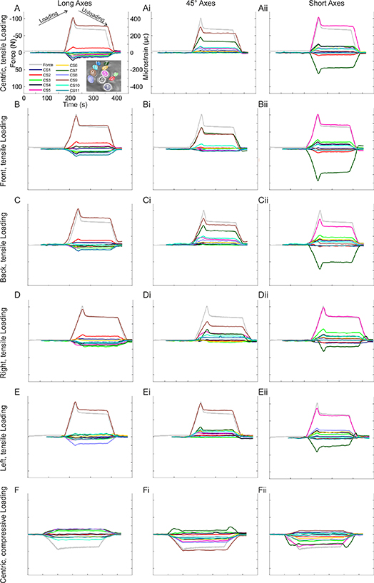
Figure 3. CS axis microstrain and model force measurements during tensile and compressive displacement; tensile displacement was tested in five tensile torque conditions (centric, front, back, right, left), compressive displacement in a centric loading condition; grey lines show monitored force; each CS has three axes (long, short, and 45° in elliptical CS and BRTL [bottom right, top left], BLTR [bottom left, top right], and 45° in more circular CS) whose changes in resistance were monitored; (A)–(Aii) tensile displacement, centric loading case; (A) long axes; (Ai) 45° axes; (Aii) short axes; (B)–(Bii) tensile displacement, front loading condition; (B) long axes; (Bi) 45° axes; (Bii) short axes; (C)–(Cii) tensile displacement, back loading condition; (C) long axes; (Ci) 45° axes; (Cii) short axes; (D)–(Dii) tensile displacement, right loading condition; (D) long axes; (Di) 45° axes; (Dii) short axes; (E)–(Eii) tensile displacement, left loading condition; (E) long axes; (Ei) 45° axes; (Eii) short axes; (F)–(Fii) compressive displacement, centric loading condition; (F) long axes; (Fi) 45° axes; (Fii) short axes.
Download figure:
Standard image High-resolution imageFurthermore, the constant displacement test, which exhibited varying force within the model due to stress relaxation, demonstrated the viscoelastic properties of the model (figures 4(A)–(B)). Independent of the speed of model elongation, the model showed stress relaxation when the sample length was held at a constant elongation after reaching a peak force of 100 N. Interestingly, the plateau-like phase during unloading (figures 3 and 4) decreased noticeably in duration at higher model elongation speed (figures 4(B) and (Bi)). Because the neural discharge of some CS primarily reflects the time rate of change of the force [18, 26, 61], we plotted the time rate of change of each cap's strain during these experiments (figures 4(Ai)–(Bi)). These data showed that the CS discharge may most strongly reflect the rate of change during the onset and offset of model displacement but not during viscoelastic creep.

Figure 4. Constant displacement tests at different motor speeds; motor velocity was reduced to 0 for 150 s once peak force was reached; grey lines show force measurements; (A) motor speed of 0.458 rpm; (B) motor speed of 2.29 rpm; (Ai) rate of change for each strain recording at a motor speed of 0.458 rpm; (Bi) rate of change for each strain recording at a motor speed of 2.29 rpm.
Download figure:
Standard image High-resolution image3.2. Differences between loading cases
The monitored strain differed in magnitude among the caps, between their axes (i.e., short and long), and among loading conditions (i.e. left, right, front, back, centric) (figure 3, tables 2 and 3). While monitoring the force exerted onto the model, the changes in resistance monitored by the strain gauge rosettes were converted to digital signals and further converted to microstrain (figures 3(A)–(F)). In the centric condition (figures 3(A)–(Aii)), the long/BRTL axis compressed in three CS (CS 1, 2, and 9) and elongated in eight CS (CS 3, 4, 5, 6, 7, 8, 10 and 11). In the 45° axes, nine CS compressed (CS 2, 3, 4, 5, 6, 7, 8, 9, and 10). The short/BLTR axis compressed in 7 CS (CS 3, 4, 5, 6, 8, 9, and 10) and elongated in four CS (CS 1, 2, 7 and 11). Consequently, in the centric condition, compression was seen in all three axes of some caps.
Table 3. Compression in each CS in all conditions
| CS 1 | CS 2 | CS 3 | CS 4 | CS 5 | CS 6 | CS 7 | CS 8 | CS 9 | CS 10 | CS 11 | Sum | |||||||||||||||||||||||||
|---|---|---|---|---|---|---|---|---|---|---|---|---|---|---|---|---|---|---|---|---|---|---|---|---|---|---|---|---|---|---|---|---|---|---|---|---|
| BRTL | 45 | BLTR | L | 45 | S | L | 45 | S | BRTL | 45 | BLTR | BRTL | 45 | BLTR | L | 45 | S | L | 45 | S | L | 45 | S | L | 45 | S | L | 45 | S | L | 45 | S | S | S + BRTL | S + BLTR | |
| Centric | x | x | x | x | x | x | x | x | x | x | x | x | x | x | x | x | x | x | x | 5 | 6 | 7 | ||||||||||||||
| Front | x | x | x | x | x | x | x | x | x | x | x | x | x | x | x | x | x | x | x | x | 4 | 6 | 7 | |||||||||||||
| Back | x | x | x | x | x | x | x | x | x | x | x | x | x | x | x | x | x | x | x | x | x | 5 | 6 | 7 | ||||||||||||
| Right | x | x | x | x | x | x | x | x | x | x | x | x | x | x | x | x | x | x | x | x | x | x | 6 | 7 | 8 | |||||||||||
| Left | x | x | x | x | x | x | x | x | x | x | x | x | x | x | x | x | x | x | x | x | x | 4 | 4 | 7 | ||||||||||||
| Comp. | x | x | x | x | x | x | x | x | x | x | x | 2 | 4 | 3 | ||||||||||||||||||||||
| Sum | 4 | 4 | 3 | 5 | 5 | 0 | 1 | 5 | 5 | 1 | 5 | 5 | 2 | 4 | 5 | 1 | 4 | 5 | 3 | 6 | 0 | 1 | 5 | 5 | 5 | 5 | 4 | 1 | 5 | 6 | 0 | 3 | 1 | |||
Compression along the indicated axis marked by x; centric, front, back, right, left represent loading conditions; Comp., compression; CS, campaniform sensilla; L., long axis; 45., 45° axis; S., short axis; BRTL 'bottom right, top left'; BLTR 'bottom left, top right'.
In each loading condition, a unique pattern of CS strain emerged. Compared to the centric loading condition, the front loading condition compressed more CS along their long/BRTL axes (5 total); one CS fewer along their 45° axes (8 total); and the same amount along their short/BLTR axes (7 total). The back condition compressed the same amount of CS the long/BRTL axis (3 total); two CS more along the 45° axis (11 total); and the same amount along the short/BLTR axis (7 total). The right loading compressed one CS more along the long/BRTL axis (4 total); one more along the 45° axis (10 total); and one more along the short/BLTR axis (8 total). The left condition compressed one CS more along the long/BRTL axis (4 total); one CS more along the 45° axis (10 total); and the same amount of CS along the short/BLTR axis (7 total). Compared with the tensile centric loading condition (figures 3(A)–(Aii)), the compressive centric loading condition (figures 3(F)–(Fii)) compressed two CS more along the long/BRTL axis (5 total); six CS fewer along the 45° axis (3 total); and four CS fewer along the short/BLTR axis (3 total). This underlines that the short axis compression counts are similar between all cases, with only right loading compressing one more CS than the other cases. However, all loading cases do not compress the same CS along the short axis and the loading cases differently affect the compression rates along the 45° and long/BRTL axis.
3.3. Short axes compression
Because CS discharge appears most sensitive to compression along its short axis [10, 44], we plotted the responses along the short axis for all tensile loading conditions and each CS (figure 5). Some CS (CS 2, 3, 4, 5, 6, 7, 8, and 10) showed the same sign of response to displacement in each loading condition. CS 2 and 7 elongated in every case, while the remaining six CS consistently compressed (although with different amplitudes in each case). The remaining CS (CS 1, 9, and 11) showed responses of varying sign in each loading condition. CS 1 compressed during left, front, and centric loading, but elongated during back and right loading. It should be noted that in one out of three trials, CS 1 compressed during front and left loading and elongated in back, right, and centric loading (Supp. Table 1). CS 9 compressed during back, right, and centric loading, but elongated during front and left loading. Interestingly, this elongation arose after a short compressive phase during force increases, suggesting that insect CS fields may also exhibit rich temporal dynamics. CS 11 compressed during right loading and elongated in all other conditions.

Figure 5. Analysis of short axis displacements during each loading scenario; (A–Ax) all caps, aligned as seen in the organism, showing monitored microstrain in all loading scenarios; (A) CS 11; (Ai) CS 7; (Aii) CS 10; (Aiii) CS 6; (Aiv) CS 3; (Av) CS 9; (Avi) CS 5; (Avii) CS 2; (Aviii) CS 8; (Aviiii) CS 4; (Ax) CS 1.
Download figure:
Standard image High-resolution image3.4. Absolute change in cap shape
When the change in microstrain was transformed into changes in length measured in pixels and this was applied to the original ellipse shape, the displacement was shown to affect ellipse shape (figures 6(A)–(E)). During centric loading, the greatest displacement was seen in CS 5, 7, and 9. However, changes were present in all CS throughout the field. Similar displacement patterns were seen during front and back loading (figures 6(B) and (C)). There is a decrease in displacement in CS 7 in right (figure 6(D)) and left (figure 6(E)) loading. In all loading conditions, it was apparent that the caps could shear, as the axes with the largest displacement were not necessarily aligned with the major or minor axes of each ellipse. When the displacement was viewed in connection with changes in force occurring over time, the rate of change and the onset of change of the recorded microstrain varied during loading (Video S1–5).

Figure 6. Plots showing the total displacement at peak force and eccentricity plotted as function of absolute value of change; (A-E) schematics showing the effects of changes in axis length induced by displacement at peak force; original cap outlines were extracted from scanning electron image, their axes are plotted with filled lines; displaced axes are dotted; changes in cap shape shown with dotted lines; all displacement effects were amplified and have the same scaling; color represents total displacement at peak force (A) centric loading; (B) front loading; (C) back loading; (D) right loading; (E) left loading. (Ai–Ei) plots showing the eccentricity of each cap against the absolute value of change; (Ai) centric loading; for this case, three different trials (supp. table 1) are plotted; (Bi) front loading; (Ci) back loading; (Di) right loading; (Ei) left loading; T1, trial 1; T2, trial 2; T3, trial 3.
Download figure:
Standard image High-resolution image
In all five tensile loading scenarios, CS 7 and 9 had the largest absolute changes in shape (figures 6(Ai)–(Ei)), seen during centric, front, and back loading in CS 7 (figures 6(Ai)–(Ci)) and during right and left loading in CS 9, where the absolute change was greater than in CS 7 (figures 6(Di) and (Ei)). All other CS showed changes in shape throughout displacement but to a lesser extent than CS 9 and 7. There was no clear pattern connecting eccentricity with changes in shape. The results from multiple trials with the same loading conditions (figure 6(Ai)) were similar in the degree of change in shape.
3.5. Controls
To test whether the peak force of 100 N was sufficient for testing CS responses, we increased the displacement up to a force of 170 N (figure S3, table S1). This produced results similar to those with a force of 100 N (table 4). However, the amount of monitored microstrain was, on average, higher during greater force and the consequent higher displacement, especially along the short axes (table S1). In some cases, such as with the long axis of CS 1, slight elongation was seen at 170 N (−0.56 µ ), although all values at 100 N were positive, thus showing compression. These values ranged from 2.94 µ to 7.25 µ. Similarly, in trial 1 (T1) at 100 N, there was elongation (−7.77 µ), while all other trials (T2, T3, 170 F) showed compression (positive values), ranging from 1.61 µ to 13.29 µ. Only two instances in three trials (3 trials × 11 caps × 3 axes = 99 total instances) showed tension instead of compression or compression instead of tension (table S2). Despite these occasional differences, repeated experiments showed comparable results.
Table 4. Microstrain values for each CS axis at peak force during displacement
| Long axis/BRTL | CS 1 | CS 2 | CS 3 | CS 4 | CS 5 | CS 6 | CS 7 | CS 8 | CS 9 | CS 10 | CS 11 |
|---|---|---|---|---|---|---|---|---|---|---|---|
| Front | 0.56 | 85.91 | −39.01 | −58.07 | 33.11 | −30.84 | 35.46 | −68.28 | 387.37 | −25.63 | −87.38 |
| Back | 29.39 | 65.96 | −35.58 | −16.99 | −31.5 | −27.47 | −7.21 | −73.41 | 409.68 | −5.47 | −73.63 |
| Right | 25.57 | 68.60 | −52.44 | −35.13 | −53.7 | 5.57 | −54.15 | −39.05 | 366.7 | −21.1 | −42.85 |
| Left | −3.77 | 38.94 | −28.3 | −15.11 | −30.46 | −3.13 | 20.56 | −97.83 | 404.41 | 37.64 | −34.01 |
| Centric | 3.66 | 65.15 | −37.58 | −92.96 | −35.78 | −22.78 | −13.28 | −69.35 | 407.80 | −4.74 | −59.56 |
| 45° axis | CS 1 | CS 2 | CS 3 | CS 4 | CS 5 | CS 6 | CS 7 | CS 8 | CS 9 | CS 10 | CS 11 |
| Front | 1.58 | 20.57 | 12.88 | −17.47 | −11.13 | 11.39 | 257.29 | 2.68 | 248.00 | 58.64 | −25.41 |
| Back | 29.09 | 14.98 | 8.69 | 10.02 | 82.23 | 28.58 | 220.48 | 59.24 | 300.86 | 86.63 | 4.00 |
| Right | 7.33 | 0.26 | 0.69 | 13.94 | 105.79 | −0.72 | 131.52 | 42.30 | 225.22 | 71.98 | 37.15 |
| Left | 17.39 | 16.91 | −4.51 | 68.62 | 43.71 | 69.24 | 114.70 | 58.02 | 385.18 | 85.89 | 5.43 |
| Centric | −0.63 | 19.29 | 3.04 | 25.29 | 67.91 | 15.43 | 180.03 | 47.62 | 300.92 | 72.78 | −2.58 |
| Short axis/BLTR | CS 1 | CS 2 | CS 3 | CS 4 | CS 5 | CS 6 | CS 7 | CS 8 | CS 9 | CS 10 | CS 11 |
| Front | 14.73 | −42.66 | 111.12 | 80.37 | 410.01 | 62.04 | −370.91 | 60.22 | −1.87 | 54.12 | −14.82 |
| Back | −6.14 | −22.64 | 117.22 | 62.21 | 296.44 | 66.42 | −280.47 | 55.41 | 20.00 | 33.77 | −20.17 |
| Right | −20.22 | −21.79 | 138.19 | 70.01 | 384.87 | 42.07 | −116.45 | 29.66 | 36.77 | 65.89 | 8.50 |
| Left | 22.42 | −12.26 | 58.32 | 84.39 | 345.74 | 75.38 | −157.98 | 111.23 | −15.85 | 15.68 | −12.96 |
| Centric | −7.77 | −34.54 | 92.55 | 100.90 | 415.48 | 59.90 | −244.21 | 57.41 | 24.62 | 48.02 | −8.28 |
Orange numbers are negative values (tension); blue numbers are positive values (compression); front, back, right, left, and centric represent loading conditions; outlined boxes highlight highest value along the short axis; CS, campaniform sensilla; BRTL, bottom right top left; BLTR, bottom left top right.
Reducing the complexity of the model by using a slab of cuticle-like resin without any holes as well as with a single circular hole made of the cap-like resin showed that the materials affect strain measurements (figure S1). The block without the hole and cap-cylinder showed tension along its long axis and compression along its horizontal axis. These values were higher when the force reached 400 N (figures S1(B), (C), (E), (F)). Both these control models showed non-linear responses to displacement (figures S1(Bi)–(Biii), (Ci)–(Ciii), (Ei)–(Eiii), (Fi)–(Fiii)).
4. Discussion
We utilized additive manufacturing printing with resins, strain gauges, and a tensile testing apparatus to investigate the exoskeletal components of insect strain organs and their properties during force application. This technical interface allowed us to mimic the morphology of an entire CS field and to apply different loading conditions. Crucially, this physical model introduced viscoelastic effects, which are known to affect strain sensing in vivo, but are challenging to accurately simulate using computational methods such as FEA. In the present experiments, tensile displacement of the field compressed many CS caps, while compressive displacement primarily elongated the caps. As elliptical CS should primarily discharge in response to strains that compress their short axes [75], most CS should have been active in the right loading condition. However, all other loading scenarios only compressed one CS fewer along the short axis. Subjecting our model to differently-oriented bending loads also revealed a population code of load, even in directions this field is not tuned to detect. This is a concrete hypothesis that future experimental studies may investigate.
4.1. Viscoelasticity
The viscoelastic properties of non-neuronal structures affects the neural response of the majority of mechanoreceptors [1]. Our model captures the predicted Young's moduli of D. melanogaster CS components using different resin materials. Although these resins were not a perfect model of the materials in animals, the ratios in compliance between the cap, collar, and exoskeleton were comparable to those in animals. It is also important to note that, even between individuals of the same species, the sclerotization of cuticle varies, leading to differences in exoskeletal parameters [61]. The use of resins allowed the inclusion of viscoelastic material properties, which is highly useful for modeling the stress relaxation and creep behavior of viscoelastic materials [76, 77].
Our physical model circumvented the difficulties of using FEA to calculate the deflection of parts composed of viscoelastic and nonlinear materials [76–78]. In the most basic sense, the physical model allowed the measurement of deflection without having to set parameters of the numerical calculation such as element size, element type, element density, and boundary conditions, all of which may affect the accuracy of the result [79]. As a result, the stability and accuracy of our experiments did not rely upon the assumptions that the materials are linearly elastic and the deflections are small, as the resins can be deflected to breakage. Our resin model exhibits cuticle-like [61] dynamic responses to loads (e.g., stress relaxation, creep). Simulating such responses with FEA requires the implementation of partial differential equation solvers, which complicate the process of simulating the deflection [76]. Indeed, developing fast and accurate finite element methods for calculating the responses of such materials is an active area of research [76–78]. Aside from the individual advantages of either physical or finite element modeling, both are limited by the available data. Detailed measurements of Young's moduli throughout the CS material or the orientation of chitin fibers are necessary to increase the accuracy of these models.
Exoskeletal viscoelasticity affected the measurements of strain sensors embedded within our model in the present study. Recent experiments completed in the legs of the stick insect Carausius morosus showed stress relaxation in the viscoelastic exoskeleton during constant displacement tests, over the span of hundreds of milliseconds [61]. Our model captures the stress relaxation seen in these animal experiments (figure 4). The experiments completed in the stick insect also measured the neuronal activity of CS during displacement. Constant displacement of the leg segment induced discharges in a group of CS, the frequency of which decreased sharply and transiently during the most rapid phase of stress relaxation. In contrast, during a constant-force test, no stress relaxation occurred, and instead, the cuticle exhibited creep, in which the displacement continued to grow throughout the experiment. This stimulus caused discharges in the same CS group as when the force was held constant, but without the transient discharge decrease observed in the constant displacement test. These results mean that (1) viscoelasticity is an important attribute for CS models to include, and (2) the extraction of the peak microstrain at 100 N for each axis in the present study could likely capture the displacements that lead to neuronal discharges in animals (as seen in table 4). Similarly to this study [61], where the plateau phase during energy dissipation in the cuticle was roughly 2.3 mN down to 1.7 mN (27%), the present study showed similar relaxation with a peak force of 100 N and a plateau phase force of about 80 N (20%, figure 4).
In some loading conditions, such as right loading (figures 3(D)–(Dii)), some CS were under tension during force increases and decreases but were under compression during peak force and the subsequent plateau phase (e.g. CS 7). Such responses may be due to the interplay of the holes within the structure, with changes in compression in one CS propagating to neighboring CS, as well as to the effects of viscoelasticity. This could also imply that the monitored rate of force in CS could be a purely mechanical consequence, which is strongly indicated in figure 4. Along this line, we also saw differences in the onset of compression and tension in different CS (Video S1–5), which suggests that CS fields detect load in a fundamentally dynamic way. Animal experiments are needed to confirm that this form of strain propagation is present in the animal and to test whether such propagation has functional impact on behavior.
4.2. Cap shape
Cap size acts a filter for force [41, 60], which allows the system to fractionate signals through the sensitivity of CS with different cap sizes. Smaller CS fire at lower loads than larger CS [51]. Additionally, cap size determines the amount of possible displacement. One study showed that greater width-to-length ratios in cuticular holes led to higher deformation [60]. The largest ratio was in the circular CS (CS 1, 4, 5). The smallest ratio was seen in CS 3, followed by CS 10 and 2. Although CS 3 had comparably high microstrain values in all 5 cases along its short axis, these values were lower than the compressive microstrain seen in CS 4 and 5. This may be due to the amplifying collars that CS 1, 4, and 5 have. In this regard, CS 5 compressed along its short axis in all loading cases with the highest microstrain values of any CS. The largest ratio amongst the elliptical CS is found in CS 7 and 8. Compared to these CS, CS 3 has larger compressive short axis microstrain in all loading cases, except during left loading, in which its microstrain value is lower than in CS 8. However, CS 10 only has higher microstrain values than CS 9, not CS 8 except during right loading. Thus, in this model, cap ratio is not sufficient for predicting microstrain strength. Factors such as position within the field, collars, and the cuticle morphology may contribute to microstrain intensity.
Plotting the absolute change in cap shape against the eccentricity of the CS extracted from a scanning electron microscope image showed that CS 7 and CS 9 consistently had the largest absolute values of change (figure 6). CS 9 has the lowest eccentricity and CS 7 the fourth highest eccentricity of all elliptical CS. Similarly, to CS 5, which had the highest absolute changes from the circular CS in the majority of loading scenarios, CS 9 is in a similar location within the field. Both are second-most distal CS within their respective column, and in proximity of the most extruded part of the model. CS 7 on the other hand is the most proximal CS of its respective column. This also means its closest to the attachment sites of the model to the tensile tester, which may influence its displacement, albeit CS 11 has a similar proximity and did not show this. Nonetheless, different loading cases differently affected the absolute changes in cap shape, suggesting that eccentricity alone does not determine the effects on cap shape.
Conclusively, these findings suggested that, in the femoral field, CS cap size or eccentricity may not directly affect the amount of displacement that occurs. We believe that the axis ratio of the caps does not necessarily predict the degree of displacement in physiological models, where the surrounding cuticle provides discontinuities that affect strain distribution. In addition to this, we also observed CS undergoing shear more frequently than a change in short-to-long axis ratio (e.g. CS 10, 9, and 1 in centric loading; figure 6). How this affects CS discharges, or rather if this is sufficient to evoke neuronal discharges, remains unclear, and must be addressed with animal experiments.
4.3. CS orientation
The femoral field CS are arranged in three columns, with the elliptical CS having the same long axis orientation in each column. The field has four elliptical CS with the same orientation and a further four elliptical CS with a mirrored orientation. This suggests functional grouping, as these CS should exhibit similar directional sensitivity [21, 51, 80]. The long axes of all of these elliptical CS are at a 45° angle to the long axis of the femur, which should make them sensitive to torques about the long axis of the leg [44], which we cannot directly apply with our experimental setup.
CS 2, 3, 6, and 7 have similar short axis orientation, with CS 8, 9, 10, and 11 having a mirrored orientation. In the first group (CS 2, 3, 6, 7), two out of the four CS compressed during all loading conditions, while the other two elongated. CS 2 and 6 showed the largest microstrain during left loading, CS 3 and CS 7 during right loading. In the other group (CS 8, 9, 10, 11), we saw similar differences. CS 8 had the highest microstrain during left loading, and CS 9–11 during right loading. Thus, independent of the proposed functional group, CS from Group 1 and Group 2 appear most sensitive to the same stimuli (table 4).
All elliptical CS had the largest microstrain values during left (CS 2, 6, 8) or right (3, 7, 9, 10, 11) loading.
This highlights that (1) left and right torques stimulated the elliptical CS most intensely, and (2) the directionality of the axes do not necessarily determine to which torques they are most sensitive. This was likely caused by various factors. For example, the long axes from each CS in the functional units are not precisely aligned within the animal or in our model. This, in combination with the aforementioned complex structure of the cuticle, may lead to differences in sensitivity. Further, the nano-CT segmentation used to create our physical model only included a small section of the cylindric femur. In a full cylinder, stresses may be distributed around the circumference (i.e., hoop stress) that couple and constrain the strains perpendicular to the loading axis on the lateral edges of our model. Additionally, left and right torques applied at a greater distance from the field may amplify the effects by increasing the rotational forces working on functional subsets.
Interestingly, the heatmaps highlighting change in shape (figure 6) suggest that the greatest change, besides the previously described effects on CS 7, is seen in CS 9 and 5, which are within one row, not one column. CS 9 has the greatest microstrain along its long axis in all loading conditions compared to all other CS, and CS 5 has the highest microstrain along their short/BRTL axis in all loading conditions. This differs from the FEA study of this field [30], in which the modeling results suggested that there is a distal to proximal gradient in displacement, with the greatest change in the most distal CS. However, the authors also showed that the removal of all sockets increases the displacement throughout the field, with the greatest effect on the second most distal CS of each column (CS 4 and 9), and a gradient effect to the third most distal CS (CS 10 and 5). It must be noted here that, due to the interconnected sockets in that study, the columns were defined as CS 1, 4, 5, 6 and CS 8, 9, 10, 11. In the current study, we are defining them as CS 1, 2, 3; CS 4, 5, 6, 7; and CS 8, 9, 10,11. They concluded that the sockets affect the overall compliance of the field. This current mechanical model does not include any sockets, which may contribute to the differences that we see. Additionally, these CS are amongst the largest of the field, surrounded by multiple CS, and close to the aforementioned most extruded area of the model. All of these attributes may contribute to their increases in the measured strain relative to the FEA model.
Control experiments further underlined the strong effects that the cuticle heterogeneity has on strain sensing. The cuticular slab control model showed compressive and tensile strains, while the cuticular slab model with an elastic cylindrical inlet did not. The complexity of the field, with the interplay of various caps, cuticular holes, and cuticle shape and thickness, affects CS strain. Previous investigations have shown that cuticle heterogeneity could alter the sensitivity of a cap to stress [35], with material discontinuities affecting the concentration and amplification of strain throughout an area [8]. The viscoelasticity of the cuticle in combination with holes that essentially reduce the amount of material affected by changes in position and the strain working on CS can lead to sensing of rates of change [41].
4.4. Study limitations
This study simplified several details of the animal in order to better understand how CS fields function. The model consisted of a simplified CS field without sockets. Previous studies have shown that sockets may act as interconnected units that themselves have an axis of compression [30]. The missing sockets may reduce the strains experienced by the CS, and the accuracy of future models would be increased by their inclusion. Furthermore, the Young's moduli used as reference are assumptions made for Calliphora vicinia [35], a blow fly that is in the same order as D. melanogaster, but the values in D. melanogaster have not been measured and may differ. We believe that the Young's moduli in our model still reflect the heterogeneity of the insect cuticle. Additionally, the caps in animals consist of two different materials [8, 37]. Here, only the more elastic of the two was included. In this regard, although the artificial exoskeleton created here reflected the viscoelastic properties of the natural materials, the exoskeleton in insects consists of various layers, each with different elastic properties. These differences may contribute to differences in compression and tension [81].
A further limitation is the difficulty of engineering the model and its instrumentation. Amplifying 33 highly-sensitive recordings simultaneously introduced the possibility of sensor failure and electrical interference, and both hardware (e.g. shielding) and software (e.g. signal filtering) solutions were necessary for successful data collection. We did see minor differences between different trials (table 4), which may be due to environmental conditions (e.g. temperature, humidity) affecting circuitry and thus recordings or to the effects of loading on the model itself, such as plastic deformation. Moreover, the exact orientation of each strain gauge, and minute variations in orientation after replacing broken sensors, is prone to human-induced variability. Consequently, this made this line of experiments expensive, which may hinder their repeatability in general. However, we believe there are positive tradeoffs and long-term benefits to the approach we took. First, the strain sensors we used were costly, but alternative methods for studying skeletal strain such as FEA also have costs in the form of time to learn the theory, time to learn the tools, computer hardware, and computational time, so we believe both these methods and more are needed to best understand how CS fields function in vivo. In future work, we plan to develop custom, miniaturized sensors with all the strain gauges attached, improving the reliability of sensor placement and orientation. Finally, we have already begun exploring how the distributed sensing of a CS field can improve strain measurement on the legs of a walking robot, both by increasing resilience in the face of sensor failures and robustness in the face of signal noise. Building the physical model in this study has forced us to confront these issues and find solutions for future applications.
Correlating monitored strain with cellular activity is not trivial. A study by Menon et al [41] suggested that a displacement of 1 nm may be sufficient to elicit CS discharges. The dynamic firing model from Szczecinski et al [19] was capable of estimating neuronal discharges from strain gauge measurements; however, this model was based on the cellular properties of stick insect CS in the tibia. We do not know how the cellular properties the femoral CS in D. melanogaster may differ from these. Future experiments should, nonetheless, attempt the conversion of microstrain to neuronal firing, either through modeling or biological experiments such as calcium imaging.
5. Conclusions
We manufactured a 3-dimensional printed resin model, with different material compliances, to investigate the response properties of an insect strain organ to applied force. This model captured differences in strain sensing induced by morphological characteristics. Different stimuli with differing degrees of compression and tension evoked changes in cap shape, which would alter CS responses. This study provides a basis for future investigations into the interplay of the cuticle and strain sensing.
Acknowledgments
We would like to thank the Lane Innovation Hub for support, tools, and equipment. We would also like to thank Sasha N. Zill and Alexander S. Chockley for feedback on the manuscript.
Data availability statement
The data that support the findings of this study are openly available at the following URL/DOI: https://doi.org/10.33915/datasets.2 [82].
Author contributions
GFD: experimental design, conceptualization, 3D printing, data collection, data analysis, figures, funding acquisition, manuscript writing and editing; WPZ: experimental design; AL: 3D printing; JF: 3D printing, conceptualization; NSS: experimental design, conceptualization, data analysis, funding acquisition, manuscript writing and editing.
Funding
WPZ and NSS were supported by NSF DBI 2015317 as part of the NSF/CIHR/DFG/FRQ/UKRI-MRC Next Generation Networks for Neuroscience Program. WPZ and NSS were supported by NSF IIS 2113028 as part of the Collaborative Research in Computational Neuroscience Program. GFD was supported by DFG DI 2907/1-1 (Project Number 500615768).
Conflict of interest
The authors declare no conflicts of interest.
Supplementary data (0.8 MB PDF)
S1-DispCentric (7.5 MB AVI)
S2-DispFront (7.3 MB AVI)
S3-DispBack (7.3 MB AVI)
S4-DispRight (7.5 MB AVI)
S5-DispLeft (7.5 MB AVI)