
Abstract
Previous studies suggested that wing pitching, i.e. the wing rotation around its long axis, of insects and hummingbirds is primarily driven by an inertial effect associated with stroke deceleration and acceleration of the wings and is thus passive. Here we considered the rapid escape maneuver of hummingbirds who were initially hovering but then startled by the frontal approach of a looming object. During the maneuver, the hummingbirds substantially changed their wingbeat frequency, wing trajectory, and other kinematic parameters. Using wing kinematics reconstructed from high-speed videos and computational fluid dynamics modeling, we found that although the same inertial effect drove the wing flipping at stroke reversal as in hovering, significant power input was required to pitch up the wings during downstroke to enhance aerodynamic force production; furthermore, the net power input could be positive for wing pitching in a complete wingbeat cycle. Therefore, our study suggests that an active mechanism was present during the maneuver to drive wing pitching. In addition to the powered pitching, wing deviation during upstroke required twice as much power as hovering to move the wings caudally when the birds redirected the aerodynamic force vector for escaping. These findings were consistent with our hypothesis that enhanced muscle recruitment is essential for hummingbirds' escape maneuvers.
Export citation and abstract BibTeX RIS

Original content from this work may be used under the terms of the Creative Commons Attribution 4.0 license. Any further distribution of this work must maintain attribution to the author(s) and the title of the work, journal citation and DOI.
1. Introduction
Studying the torque and power requirements for wing actuation in the flight of hummingbirds is useful for understanding the muscle functions and biomechanics that enable their wing motions, and it could also provide helpful guidance for man-made flapping-wing flyers inspired by such creatures. Like other animal flyers, hummingbird wings are capable of three degrees-of-freedom rotation at the shoulder joint, namely stroke, pitch, and deviation. Among these three, stroke usually requires the most torque and power inputs from the flight muscles to accelerate the wings and overcome the aerodynamic resistance. Along with the stroke motion, the wings have to rotate back and forth around their longitudinal axis. Such pitch rotation is a critical kinematic factor of flapping wings in general [1], and thus its mechanics and actuation also require attention for refining experiments in bio-inspired robotics [2–4].
Pitch rotation allows the wings to operate at an effective angle of attack relative to the air at a given instantaneous stroke velocity (also referred to as wing translation) for lift production. For flyers such as many insects and hummingbirds whose wings move mostly in a horizontal plane while hovering, an almost complete pitch reversal of the wings around the end of downstroke is necessary to maintain a positive angle of attack for upstroke to generate additional weight support. For hummingbirds, upstroke produces only about half of weight support as downstroke [5–7] yet is still considered key to their ability to sustain hovering flight. When combined with the stroke motion, dynamic pitching of the wings helps generate unsteady lift through mechanisms such as rotational circulation, delayed stall, and accompanying leading-edge vortices to further enhance lift production for those hovering flyers [8–12].
Pitching dynamics of a flapping wing is affected by the wing's own inertial force, the aerodynamic force acting on the wing, and input from the muscular system of the animal. Since the wing's center of mass is behind the longitudinal axis, the inertial force associated with stroke reversal tends to pitch the wing and cause it to flip around the longitudinal axis. By estimating this inertial force for flies, Ennos [13] concluded that the wing inertia is sufficient to drive the pitch reversal and thus wing pitching could be passive (i.e. there is no need for active input from the flight muscles). Bergou et al [14] further studied wing pitching of various hovering fruit flies, dragonflies, and hawkmoths using computational fluid dynamics (CFD) as well as a quasi-steady model to resolve both inertial and aerodynamic forces. They also concluded that no net power is required from those insects for the pitch reversal, thus suggesting that the wing pitching mechanism could be completely passive. A recent study of Ruby-throated hummingbird by Song et al [15] using CFD to simulate the detailed aerodynamic forces showed that the pitch reversal of hovering hummingbirds was also driven by wing inertia; however, there were clear indications of power input for pitch-up of the wings during downstroke that was instrumental for lift production. Despite the finding, their results were not sufficient to suggest that such power supply was from active muscle input since the net power input in a complete wingbeat cycle was still negative for wing pitching. Note that a passive spring mechanism due to elastic energy storage in connective tissue associated with the flight muscles would potentially be able to store energy from pitch reversal that is driven by inertia and then release the energy to power the pitch-up movement [16].
From a physiological perspective, hummingbirds possess a sophisticated musculoskeletal system that is substantially different from insects and is capable of active wing pitching at the shoulder joint [16, 17] or even wrist joint [17]. Moreover, we generally hypothesize that steady-state behaviors should be dominated by efficiency, while an unsteady maneuver such as escaping from threatening stimuli may rely on efficacy, with the need to survive superseding the need to minimize energetic costs [18–20]. Thus, we hypothesized that active muscle contributions should increase in relative importance during threatening situations for hummingbirds [18–20] and this may include active wing pitching. To test this, we have investigated the wing mechanics of the escape maneuver by startled hummingbirds. We focused on the escape maneuver because it represents an extreme mode of flight where hummingbirds likely maximize their maneuvering capability and power output in such situations for the sake of safety.
It has been found that the wing kinematics in the hummingbirds' escape maneuver is very different from that of hovering flight. For example, the wingbeat frequency is increased by 40%, and the wing trajectory is substantially altered in the 3D space; in addition, there are significant left-right asymmetries and temporal changes in the stroke, pitch, and deviation angles [21, 22]. Hummingbirds rely on those changes to generate maneuvering forces and torques necessary for the linear acceleration and three degrees-of-freedom body rotation [21, 22]. From a scaling point of view, when the wingbeat frequency f and corresponding stroke velocity V are increased proportionally, both the inertial force and the aerodynamic force of the wings should increase as  . Since their action points are behind the longitudinal axis, the inertial force tends to pitch up and flip the wing at the end of the stroke, thus requiring negative power input for pitching, while the aerodynamic force tends to cause the wing to pitch down at mid-stroke with maximum wing speed [13], thus requiring positive power input for mid-stroke pitching up. As a result, it is not immediately clear whether the net power requirement over a wingbeat cycle would change its sign or not since both positive power and negative power from different phases will increase accordingly with the wingbeat frequency. More importantly, temporal variations such as instantaneous wing velocity and modulation of pitching in the process could make the situation more elusive. Therefore, it is necessary to examine the detailed wing mechanics of the maneuvering flight and study its potentially different actuation mechanisms from that in hovering.
Recently, we completed a 3D CFD study of the escape maneuver using realistic wing kinematics reconstructed from high-speed videos of escaping hummingbirds [23]. In that study, our focus was on the flight mechanics of the maneuver including linear translation and pitch, roll, and yaw rotations of the bird body. Both the wing inertial forces and aerodynamic forces were calculated in that study for detailed flight analysis. In the current study, we used those force data to further calculate the torque components of the wings and also the required input torque to actuate the wings in all three degrees of freedom. The power requirement for each of those degrees of freedom was then a straightforward result. In the following sections, we briefly summarize the technical approach and then describe the results.
2. The rational-dynamics model
Two male Rivoli's hummingbirds (Eugenes fulgens) were the subjects of the current study. Their morphological data are given in table A.1 in appendix
2.1. Reconstruction of wing kinematics and CFD simulation
We reconstructed wing and body kinematics using high-speed videos of hummingbird escape maneuvers (figure 1(A)) that were described in a previous experiment of Cheng et al [21]. Briefly, the flight experiment was carried out in an acrylic plastic-made transparent chamber. Each bird's body and wings were marked with 1.5 mm water-soluble non-toxic white paints. When hovering and feeding from a syringe feeder, the bird was startled using a looming flat plate approaching from the front and immediately performed the escape maneuver. For Rivoli's hummingbirds, the reaction time to the stimuli as indicated by tail flaring was 21±1.4 ms [21] (the tail flaring time is marked out in the unscaled plots in supplementary materials). Three synchronized high-speed cameras recorded the flight sequence from different angles at 1000 frames per second.
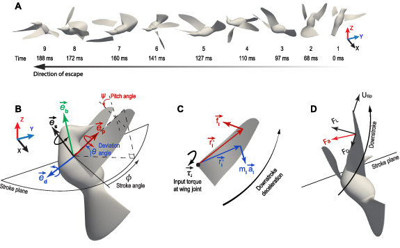
Figure 1. (A) Snapshots of the reconstructed escape flight sequence in the lab frame to show the body orientation; (B) definitions of wing stroke angle, φ, deviation angle, θ, and pitch angle, ψ, as well as axes of rotation; (C) balance of the inertial torque, aerodynamic torque, and input torque at the wing joint,  , when the right wing was decelerating at late downstroke; (D) illustration of the aerodynamic force Fa
, lift FL
, and drag FD
.
, when the right wing was decelerating at late downstroke; (D) illustration of the aerodynamic force Fa
, lift FL
, and drag FD
.
Download figure:
Standard image High-resolution imageWe used a customized Matlab script [24] to digitize the marker points on the wings from the videos. Seven marker points on each wing profile were traced. We reconstructed the wing surface using these marker points and meshed it using triangular elements. We reconstructed the bird's head, trunk, and tail using the marker points placed on the trunk and identifiable features, e.g. eyes and tips of tail feathers. The reconstructed wing-body kinematics were then used as input to an in-house code based on the immersed-boundary method [25] to simulate the full-body aerodynamics. Details of kinematic reconstruction and CFD simulation were provided by Haque et al [23], which includes verification and validation of the CFD model (see appendix  (see definitions of these variables for equation (6)).

Figure 2. Pressure differential normalized by  between two sides of the wing (ventral side minus dorsal side) of a Rivoli's hummingbird (Eugenes fulgens) from the CFD study, where several snapshots in the second escape wingbeat cycle are shown; (A) upstroke and (B) downstroke.
Download figure:
Standard image High-resolution image2.2. Calculation of wing inertial forces
Mass distribution over the wing surface, i.e. the surface density, and the instantaneous acceleration of each point on the wings, were needed to calculate the wing inertial forces. For this purpose, we used the experimentally measured wing mass distribution from Ruby-throated hummingbirds (Archilochus colubris, mass M ≈ 3.2 g) [15] and scaled the data to match the body mass of the present Rivoli's hummingbirds. Since hummingbird wings consist of feathers and a musculoskeletal structure of muscles and bones [26], we separated the mass of the bony structure and distributed it along the leading edge from the root to the finger location (see supplementary materials). The linear velocity and acceleration of each mesh node on the wing were derived from the temporally interpolated positions of the wings using a finite-difference approximation [23].
2.3. Rotational dynamics of the wings
We modeled the wing base as a ball joint between the wing and the bird body, where a force and a torque were applied by the muscles on the wing to overcome the aerodynamic forces (figure 1(D)), and meanwhile provide inertial acceleration of the wing. As a result, mechanical power was transferred from the muscle to the wing through the joint to power the wing motion. To model these effects, we defined the wing joint input torque,  , the wing aerodynamic torque,
  , and the wing inertial torque,
  , and we calculated them according to following equations:

where  is the distance from the joint to the mesh node i (figure 1(C)), mi
is the mass of a mesh node on the wing,
is the distance from the joint to the mesh node i (figure 1(C)), mi
is the mass of a mesh node on the wing,  is the linear acceleration of the node, and
  is the aerodynamic force at the node (the difference between the aerodynamic forces on the two sides of the wing). Note that a negative sign was included in the definition of the aerodynamic torque. Equation (3) may be viewed as the input torque
  from the joint being equal to the sum of two output parts: the inertial torque for wing acceleration and the aerodynamic torque to overcome the air resistance.
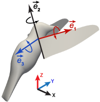
The three rotational angles of the wing were defined as below. Referring to figure 1(B), the longitudinal axis of the bird body is defined as  , and the stroke plane is defined as the plane perpendicular to
  . This definition of stroke plane is different from the one often used to describe the plane in which the wing axis roughly travels (e.g. [27]). The present definition allows us to analyze the wing movement with respect to the body and is instrumental for the discussion of wing muscle actuation when the wing trajectory is changed from hovering to escaping, especially for wing deviation. It is also useful for describing asymmetries between the two wings when the same stroke plane is consistently used. The longitudinal axis or pitch axis of the wing is defined as
  and is coincident with the first axis of the wing-fixed coordinate system
  . The stroke angle φ was defined as the angle between spanwise axis of the bird body and the projection of
  on the stroke plane. The deviation angle θ was the angle between
  and the stroke plane. The pitch angle ψ was the angle between the wing surface (viewed as a flat surface) and the plane spanned by
  and
and  . The stroke axis
  , deviation axis
  , and pitch axis
  were orthogonal axes constructed using
  and
and  . We used three points on the wing to define the wing surface plane: the wing base joint, the trailing edge corner near the wing base, and the leading ledge at the 2/3 wing span.
Note that the time derivatives of φ, θ, and ψ do not represent the angular velocities of the wing. Instead, a wing-fixed coordinate system  -
- -
- was used to define the rotational matrix and calculate the rotational velocities of the wing in this system as described in appendix
  . The angular velocity vector was then projected to each axis of the
  -
- -
- system to obtain the stroke, deviation, and pitch velocities, which were denoted as ωs
, ωd
, and ωp
, respectively.
system to obtain the stroke, deviation, and pitch velocities, which were denoted as ωs
, ωd
, and ωp
, respectively.
Then, the power input for the wing is simply the dot product between the wing joint torque  and the rotational velocity,
  so that

Note that due to the translation and rotation of the bird body during the maneuver (and thus movement of the wing joint), the wing joint force would also lead to some amount of power transfer between the body and the wing. However, this power is much smaller than the power associated with the wing rotation [23] and is thus not considered here. The individual power contributions for stroke, pitch, and deviation were defined as

The normalized power coefficient, CP , is defined as follows
Here, ρ is the density of the air, Utip is the average wing tip velocity during escape cycles, and As is the average surface area of the wing (see table A.1 for their values). This formula was used to calculate the power coefficient of the individual rotational component.
To see the net power requirement for wing pitching, the net pitch power  , the net stroke power
  , and their ratio
  were calculated for each wingbeat cycle. Furthermore, the left and right wings were also separately calculated. The separate wingbeat and single-wing calculations were done because there were significant cycle-to-cycle as well as left-right variations during the maneuver [21].
3. Results
The time-dependent stroke, pitch, and deviation angles from the reconstructed kinematics are shown in figure 3, where the left and right wings of the two birds are included, resulting in four individual data sets in addition to the averaged data. We scaled the time using the individual wingbeat period T since the wingbeat frequency was increased significantly from hovering (24 Hz) to escaping (36 Hz) and the frequencies were also slightly different between the two birds. Furthermore, downstroke and upstroke were separately scaled by their respective duration for phase-based visualization (unscaled plots are provided in supplementary materials for individual datasets). Both birds used about five wingbeat cycles ( 0 to 5) to finish the maneuver sequence of pitching up, rolling to either left or right side, and turning around to face the escape direction. A brief period of hovering (
 = −1 to 0) was also simulated as a reference. For visual understanding, the wing trajectory and instantaneous wing position are also plotted for each wingbeat cycle of one bird (figure 3 insets).
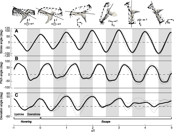
Figure 3. The averaged (A) stroke, (B) pitch, and (C) deviation angles for hovering and escape cycles in the Rivoli's hummingbird (Eugenes fulgens, n = 2). Thin-dashed lines represent angles for 4 individual data sets (left and right wings for Bird 1 and Bird 2). The thick lines represent the average. Insets illustrate the wing trajectory and change of a wing chord in a cycle.
Download figure:
Standard image High-resolution imageThe amplitude of the stroke angle was reduced at the end of upstroke in the first two cycles at  0.5 and 1.5 as compared to hovering (figure 3(A)). That is, when the birds initiated the maneuver, they terminated the upstroke earlier, and the wings' upstroke deceleration led to a backward force on the birds' body so that the body could start from a quick pitch-up rotation. This wing inertial effect on the body rotation was discussed in our recent work [23]. After initiating body pitching (
 ), the stroke angle became larger at both pronation and supination to increase wing speed and enhance force production. Pitch angle had a greater magnitude during upstroke than during downstroke (figure 3(B)). Also, the wings were much more elevated at supination, which corresponds to the backward inclination of the average wing trajectory and reorientation (figure 3(C)) of the aerodynamic force vector with respect to the body [21, 23]. These three angles defined the instantaneous position of the wings, where the required torque and power to actuate the wings were calculated as discussed next.
3.1. Torque and power for wing pitching
Individual wings had an increased pitch velocity at both pronation and supination as the hummingbirds went from hovering to escaping, although slight phase differences between the individual cases reduced the average at pronation (figure 4(A)). Especially for downstroke, the wings underwent a significantly faster pitch-up motion (positive pitch velocity) as compared to hovering, with the maximum pitch rate at mid-downstroke increasing from 100 rad s–1 during hovering to 180 rad s–1 during escaping. There were clear asymmetries between pronation and supination. Pronation took place mostly around the upstroke-to-downstroke reversal, while supination spanned much of downstroke in addition to the downstroke-to-upstroke reversal. Furthermore, the duration of pronating rotation was shorter than the duration of supinating rotation. Note that the average pitch velocity was not zero in a cycle even if the wing returned to its original position (this was due to the 3D rotation of an object). The phase and duration differences of pronation and supination led to different inertial and aerodynamic effects between them as discussed later.
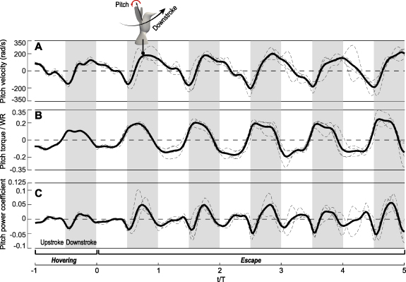
Figure 4. Pitch dynamics of the wings of Rivoli's hummingbirds (Eugenes fulgens, n = 2). (A) Pitch velocity, (B) pitch torque normalized by body weight, W × wing length, R, and (C) power coefficient Cp . The individual cases are shown as thin-dashed lines. Inset shows a wing pitching up during downstroke.
Download figure:
Standard image High-resolution imagePitch torque was significantly increased for both upstroke and downstroke after escape was initiated, with the magnitude nearly doubled from 0.1 WR to 0.2 WR (figure 4(B)); here W is the body weight and R is the wing length. Note that the pitch torque was not in phase with the pitch velocity, and when they were opposite, i.e. the pitch torque was against the pitch rotation, a negative power was produced as seen in figure 4(C) at the beginning of downstroke and also at the beginning of upstroke. Such negative power at wing reversal was also reported for hovering hummingbirds [15] (also see here the initial hovering period in figure 4(C), as well as for hovering and even maneuvering insects [14, 28]. The negative power means that these flyers need a mechanism at wing reversal to generate the reacting torque to stop the wings from continuously pitching in the same direction. Compared to hovering, the escape cycles had a greater magnitude of negative power around wing reversal. On the other hand, the downstroke of escape cycles also had much higher positive power input than the downstroke during hovering. For upstroke, the magnitude of power was much lower than that of downstroke, which was the case for both hovering and escape. In addition, only some of the escape cycles (e.g.  between 2 and 5) had significant positive power input during upstroke. The low power during upstroke was because the pitch velocity at upstroke was small (figure 4(A)) despite the corresponding torque was significant (figure 4(B)). After averaging over the individual wingbeat cycles, some cycles had positive average power input while the others had negative or nearly zero average power input (data shown later in figure 8), suggesting that active muscle activities were required to pitch the wings at least for some of these cycles.
The inertial and aerodynamic effects are plotted separately in figure 5 to further illustrate the pitching mechanism. In figure 5(A), the inertial torque peaked at wing reversals, while the aerodynamic torque peaked in the middle of each half-stroke, which corresponded to the maximum aerodynamic lift and drag at those time moments (see insets of this figure). Since lift and drag at downstroke were much higher than those at upstroke for hummingbirds [7, 23], here the aerodynamic torque also had a greater magnitude at the downstroke than the upstroke. In addition to phase differences, the aerodynamic torque became higher than the inertial torque during the escape maneuver, a situation that was different from hovering. The high aerodynamic torque, combined with high pitching velocity at downstroke as shown in figure 4(A), led to significant positive power requirement for downstroke pitching.

Figure 5. (A) The averaged inertial torque, aerodynamic torque, total input torque, and (B) their corresponding power coefficient CP for wing pitching. Insets illustrate lift and drag on the wing.
Download figure:
Standard image High-resolution imageComparing figures 5(A) and (B), the negative pitch power at wing reversals was mainly due to the inertial torque, suggesting the reversals were driven by the wing inertia. Note that here the inertial effects included not only the acceleration and deceleration of wing pitching itself but also the coupling between stroke and pitch. That is, since the center of mass of the wing is below the pitch axis of the wing, the stroke deceleration of the wing axis would cause the wing surface to continue to move forward and rotate around the axis. This coupling effect could be easily seen from the simplified rotational-dynamics equation of the wings (see appendix
3.2. Torque and power for wing stroking
Although pitch dynamics were the main focus of this work, stroke and deviation of hummingbird wings were also of our interest for comparison with wing pitch. The torque and power input for these motions could help estimate the contributions of muscle activation.
As the stroke velocity was increased from hovering to escaping, both inertial and aerodynamic torques were increased (figure 6). However, the inertial torque still had a greater magnitude than the aerodynamic torque. This comparison was different from the comparison of the pitching torques in which the aerodynamic torque exceeded the inertial torque during the escape maneuver. Therefore, these torque components did not scale exactly in the same way as the wingbeat frequency was increased because they were also affected by other changes in the wing kinematics. Stroke torque during upstroke was small and much lower as compared to downstroke (figure 6(B)). This result was caused by two factors. First, the aerodynamic forces were generally lower during upstroke than during downstroke for both hovering flight [5–7] and the present escape maneuver [23]. Another factor was the inclined wing trajectory during the escape maneuver. As the wings were moving forward and upward during downstroke (figure 6 insets), both aerodynamic lift and drag on the wings acted against the wing movement projected in the stroke plane, thus increasing the overall aerodynamic stroke torque. However, when the wings were moving backward and downward during upstroke, aerodynamic lift provided an assisting component to the wing movement projected in the stroke plane while aerodynamic drag was resisting the same movement. Thus, the two led to canceling effect and reduced the overall aerodynamic torque for upstroke. Correspondingly, the aerodynamic power as shown in figure 6(C) was much smaller during upstroke in comparison with downstroke in the first three escaping wingbeat cycles.
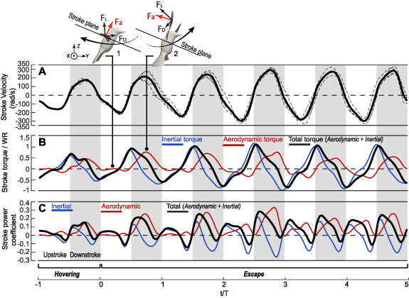
Figure 6. Dynamics of wing stroke in the Rivoli's hummingbird (Eugenes fulgens, n = 2). (A) Average stroke velocity and individual cases as thin-dashed lines, (B) torque components, and (C) power coefficients. Insets illustrate lift and drag on the wing.
Download figure:
Standard image High-resolution imageWith the aerodynamic power balancing the negative inertial power that was associated with wing deceleration, the power input for stroke in figure 6(C) was mostly positive, meaning that the input power was used to accelerate the wing stroke or overcome aerodynamic resistance, or both. The total power input was negative mainly during late upstroke, where the aerodynamic power was small and the overall power input was dominated by the negative inertial power due to upstroke deceleration. As expected, the stroke power coefficient was much higher (∼5x) than the pitch power coefficient.
3.3. Torque and power for wing deviation
To perform rapid body rotation and translational acceleration for escaping, the hummingbirds moved up their wings cranially during downstroke in the first three wingbeat cycles to redirection the aerodynamic forces as seen in figure 3 insets. On the other hand, the aerodynamic lift on the wings generally points upward and thus would help with such deviation motion (see the inset for downstroke). So it is not immediately clear whether active input was needed or not for the downstroke deviation. Figure 7(B) shows that during downstroke, the aerodynamic torque indeed helped elevate the wings, and thus the required input torque was small for the first three escape cycles. During upstroke when the wings were moving caudally in these cycles, additional torque input was needed as compared to hovering to depress the wings against both lift and drag (see the inset for upstroke). As a result, the downstroke deviation required little or even negative power input when the aerodynamic torque overcame the inertial torque to deviate the wings, while the upstroke deviation required significant power input that reached one-half of the input power for stroking during downstroke.
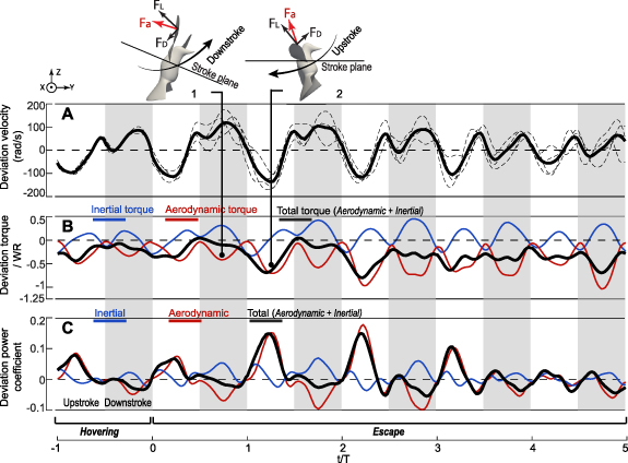
Figure 7. Dynamics of wing deviation in the Rivoli's hummingbird (Eugenes fulgens, n = 2). (A) Average deviation velocity with individual cases shown as thin-dashed lines, (B) torque components, and (C) power coefficient. Insets illustrate the effects of lift and drag.
Download figure:
Standard image High-resolution image3.4. Net power requirement for wing pitching
As shown in figure 8, the ratio of wing pitch power to stroke power,  , is scattered around zero. Left and right wings of each bird were plotted separately here because of significant asymmetries between the two wings, which were needed to control roll and yaw rotations of the body [21]. It is clear that both birds used net power for wing pitching in certain wingbeat cycles. In some of the cycles, the net pitch power may reach as much as 20% of the net stroke power. We point out that although some of the wingbeat cycles required nearly net zero or a small negative amount of pitch power, yet net positive power may still be needed in reality since the actuation mechanism is unlikely to be 100% efficient.
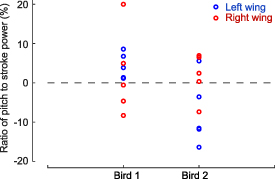
Figure 8. Ratio of wing pitch power to stroke power,  , for individual wingbeat cycles during the maneuver. The positive values suggest active pitching.
Download figure:
Standard image High-resolution image4. Discussion
It has been known that hummingbirds use drastically different wing kinematics from the hovering state to perform an escape maneuver [21]. In comparison, insects like fruit flies employ only slightly different wing kinematics from hovering to perform maneuvers [28, 29]. The drastic changes of their wing kinematics, e.g. pitch rate, deviation, and asymmetry between the left and right wings, in addition to a frequency increase of wingbeat, allow hummingbirds to greatly increase the force and/or torque production, which provide the acceleration and rotation of the body needed in the maneuvering process. Indeed, our most recent CFD study of the escape maneuver did show that the instantaneous aerodynamic force was increased by 1.9 times and power output by 2.75 times as compared to hovering [23]. It is very likely that the increased pitch rate played an important role in the process to increase the rotational lift as well as the unsteady effects associated with pitching such as the leading-edge vortices [8].
The active pitching of wings as suggested by the present study is both physiologically and energetically possible for hummingbirds. Agrawal et al [16] recently developed a comprehensive model of wing muscle functions using detailed 3D skeletal anatomy, wing joint kinematics obtained from high-speed x-ray, as well as the aerodynamic forces from CFD data. Although it was for hovering flight, their study showed that hummingbirds used their primary flight muscles, pectoralis and supracoracoideus, to power wing pitch and deviation, and that the secondary muscles were recruited only to help control these motions. Based on their findings, it is therefore expected that in the present maneuver, hummingbirds likely employed their primary flight muscles even more than hovering to empower pitching and deviation.
Hummingbirds selectively recruiting muscles of the wing to accomplish a maneuver, compared with passive pitching during steady hovering, is consistent with the 'efficiency versus efficacy' hypothesis. This hypothesis predicts that sustained, frequent locomotor activities may result in natural selection for phenotypes that maximize efficiency (mechanical work output divided by metabolic work input) whereas maneuvering for escape from potential predation should favor 'getting the job done' regardless of energetic cost [18–20]. Our modeling results lead us to predict that selection has resulted in efficiency in hovering of hummingbirds but departures from maximal efficiency to accomplish maneuvers in response to a perceived threat. This prediction merits future study in a comparative, evolutionary context to better understand the role of selection on energy use in locomotion [20].
The present findings should be useful for the design of biomimetic micro air vehicles (MAVs) that are based on flapping wings. If a passive approach were all that the MAV needs to realize the pitch rotation of the wings, then the vehicle design would be much simpler, as a spring system (and a stop mechanism, if necessary, to avoid over-pitching) may be used to temporarily store the inertial energy available from wing deceleration near a wing reversal and then release it later to pitch the wing in the opposite direction. Such an elastic mechanism could be introduced into a structural component at the wing base, or integrated into the flexible wing structure to allow twisting deformations and thus effective pitching. Indeed, some current MAVs took advantage of the idea of passive pitching and were able to greatly reduce the complexity of the wing design [30, 31]. However, our study shows that, to generate high power output and achieve high maneuverability like hummingbirds, one may need to consider introducing an active mechanism to power wing pitching in the middle of wing strokes. Of course, such an active mechanism may be combined with the passive mechanism and thus still take advantage of the available inertial energy from temporary wing deceleration so that the overall design is energy-efficient. It is noted that in several available MAV prototypes, active mechanisms have been incorporated into the wing design [2, 3, 32] to control wing pitching. These mechanisms may be further explored to enhance the maneuverability of the MAVs.
5. Conclusion
Our computational model based on high-fidelity CFD simulations showed that hummingbirds actively pitched their wings during the escape maneuver and the overall power requirement in a wingbeat cycle could be positive for the pitch actuation, suggesting that there was a net power input from their flight muscles to drive the pitch movement. Such active pitching was likely to increase the aerodynamic force production needed for the maneuver. Lastly, the drastic wing deviation also required a large amount of net power input. Support data of the CFD model have been provided [33].
Acknowledgment
This research was supported by a grant from the Office of Naval Research (ONR) (Program Officer: Dr Marc Steinberg; award number: N00014-19-1-2540) to BC, BWT, and HL.
Data availability statement
The data that support the findings of this study are openly available at the following URL/DOI: https://doi.org/10.7910/DVN/9IOAQ1.
Appendix A: Morphological data and summary of the CFD simulation
For the CFD simulation, the 3D viscous incompressible Navier–Stokes equation was solved on a nonuniform Cartesian grid using an immersed-boundary method [34]. The computational domain was a rectangular box measuring 24×21×24 cm3. Domain translation was used to follow the overall shifting position of the bird body, with the corresponding non-inertial effect incorporated into the governing equation. The baseline simulation used a total of 293 million (700×600×700) mesh points, with a time-step size of  = 5 µs. This allowed for approximately 7000 steps to resolve a complete wingbeat cycle during the maneuver. The simulation was performed using a total of 1000 processor cores on Stampede 2 at the Texas Advance Computing Center (TACC). Mesh refinement and domain size were verified in separate simulations to ensure that the mesh and domain setup were adequate. Details were included here in supplementary materials. The aerodynamic force
  exerted at each wing mesh node was simply equal to the local stress multiplied by the surface area the node occupied on the mesh.
Table A.1. Morphological data of the two Rivoli's hummingbirds used in this study.
| Parameter | Bird 1 | Bird 2 |
|---|---|---|
| Mass, M | 7.73 g | 7.49 g |
| Average cord length, c | 1.72 cm | 1.74 cm |
| Average wing surface area, As | 11.42 cm2 | 11.74 cm2 |
| Wing length, R | 7.47 cm | 7.26 cm |
| Average wingtip velocity, Utip | 10.97 m s−1 (hovering), | 11.70 m s−1 (hovering), |
| 16.23 m s−1 (escape) | 17.76 m s−1 (escape) | |
| Wingbeat frequency, f | 24.76 Hz (hovering), | 22.73 Hz (hovering), |
| 34.41 Hz (escape) | 37.75 Hz (escape) | |
| Density of the air, ρ (at 20 ∘C) | 1.204 kg m−3 | 1.204 kg m−3 |
Appendix B: Rotational velocities of the wings and the inertial effects
Figure B.9 shows the wing-fixed coordinate system, where  ,
,  , and
, and  were unit vectors along the axis 1, 2, 3 respectively. Here, axis 1 is along the pitch axis of the wing; axis 2 is along the wing cord perpendicular to axis 1, and axis 3 is obtained from the cross-product of
  and
and  . These unit vectors can be written with respect to the global coordinates such as
  , and so on. The rotational matrix Q can be constructed as below,
The rotational matrix Q transforms a vector  defined in the global coordinate system to the wing-fixed coordinate system as
  . Then, the rotational velocity of the wing,
  can be calculated using the time derivative of the rotational matrix Q as [35]
Here,  represents the cross product operator, QT
is the transpose matrix of Q, and ω1, ω2, and ω3 are the angular velocity component in axis 1, 2, 3, respectively. The time derivative of Q was computed numerically.
represents the cross product operator, QT
is the transpose matrix of Q, and ω1, ω2, and ω3 are the angular velocity component in axis 1, 2, 3, respectively. The time derivative of Q was computed numerically.
Figure B.9. Illustration of the wing-fixed coordinate system.
Download figure:
Standard image High-resolution image
To see how qualitatively the stroke acceleration/deceleration creates an inertial effect in wing pitching, we may approximate the wing as a flat plate. Its rotational dynamics in the wing-fixed coordinate system can be written as

where  ,
,  are the input torque at the wing joint and aerodynamic torque (exerted by the wing on the air), respectively, as defined in (3), and I is the moment of inertia matrix,
Since  for a flat thin plate and
  , the pitching component, i.e. the ω1 component, of the equation becomes

Stroke deceleration typically corresponds to a negative  and thus will lead to an increase in ω1.
Supplementary data (3.6 MB PDF)