

Abstract
In this work, we proposed a bar-joint model based on the corrected resistive force theory (CRFT) for studying artificial flagellated micro-swimmers (AFMSs) propelled by acoustic waves in a two-dimensional (2D) flow field or with a rectangular cross-section. Note that the classical resistive-force theory for 3D cylindrical flagellum leads to over 90% deviation in terminal velocity from those of 2D fluid-structure interaction (FSI) simulations, while the proposed CRFT bar-joint model can reduce the deviation to below 5%; hence, it enables a reliable prediction of the 2D locomotion of an acoustically actuated AFMS with a rectangular cross-section, which is the case in some experiments. Introduced in the CRFT is a single correction factor K determined by comparing the linear terminal velocities under acoustic actuation obtained from the CRFT with those from simulations. After the determination of K, detailed comparisons of trajectories between the CRFT-based bar-joint AFMS model and the FSI simulation were presented, exhibiting an excellent consistency. Finally, a numerical demonstration of the purely acoustic or magneto-acoustic steering of an AFMS based on the CRFT was presented, which can be one of the choices for future AFMS-based precision therapy.
Export citation and abstract BibTeX RIS

Content from this work may be used under the terms of the Creative Commons Attribution 4.0 licence. Any further distribution of this work must maintain attribution to the author(s) and the title of the work, journal citation and DOI.
1. Introduction
1.1. Background
An artificial micro-swimmer normally refers to an object synthesized at the microscopic scale [1, 2] and capable of interacting with a fluidic environment to achieve locomotion. While natural micro-swimmers, i.e. microorganisms, have been studied since the invention of Leeuwenhoek's microscope in the 17th century, artificial micro-swimmers were not thought possible until Richard Feynman's famous lecture [3] on nanotechnology in 1959. Since then, people have fantasized about tiny untethered robots [4] to kill bacteria and implement targeted therapy in vivo. For example, a swarm of micro-swimmers actuated by acoustic power can swim along the intestinal tract to kill the cancer cells by generating heat under an alternated magnetic field (i.e. magnetic thermotherapy), as illustrated in figure 1. Nevertheless, these tasks are still very challenging, and most of the achievements are limited to laboratory studies [5, 6] where the micro-robots appear in diverse structures, such as bubbles [7, 8], nanorods [9, 10], helical filaments [11, 12], and flagella [13, 14]. In this work, we focus on artificial flagellated micro-swimmers (AFMSs).
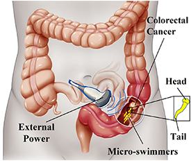
Figure 1. Schematic of a medical application of AFMSs.
Download figure:
Standard image High-resolution imageAn AFMS usually consists of a relatively rigid head and a flexible tail, as shown in the inset of figure 1, where the tail is customarily called a flagellum in microbiology [15]. We focus on the flagellated structure, especially the sperm-like one, because it is easy to fabricate through 3D printing [14] and is suitable for medical applications due to the potential of cargo transportation by its head [16]. Various actuation strategies have been proposed for artificial micro-swimmers, which can be classified into two categories [17]: the self-propulsion approaches, e.g. the catalytic reactions [18], and external actuation approaches, such as optical [19], thermal [20], magnetic [21], and acoustic actuation [22]. For AFMSs and considering medical applications, the acoustic and magnetic actuations are the most suitable because they are tissue- and circulation-friendly and have been employed in diagnosis and therapies [23]. Here we choose acoustic excitations for propulsion and navigation and also consider magnetic power to assist turning.
1.2. Micro-swimmer models and their verification
It is noted that the inertia of flagella and surrounding fluids can be ignored because the Reynolds number is sufficiently low at the microscale and when the dynamic response is away from resonance [24]. In a low Reynolds number (LRN) regime, the Navier–Stokes equation can be recast into the linear Stokes equation [25] and the linearity of the Stokes equation leads to the so-called Purcell's scallop theorem [26] which forbids objects with a reciprocal motion from moving. Instead, a traveling wave in a flagellum can generate net propulsion [27]; hence, whipping the flagellum of a micro-swimmer can propel itself forward. One may note that the strong acoustic streaming around the sharp edges is a well-established mechanism for propelling acoustically actuated swimmers [28, 29]. To simplify the swimming problem, as described by Liu and Ruan [24], the effect of actuation (e.g. an acoustic power) is simplified to actuation forces and torques on the head of a flagellated micro-swimmer, which leads to flagellum wiggling and propulsion. However, the expressions for fluid forces on a solid body are normally so complicated that numerical simulations are necessary to predict the locomotion [30]. Fortunately, if a body is slender (i.e. the ratio of the characteristic width to length is less than 0.1 [31]), an asymptotic expression in terms of the slenderness can be obtained, known as the slender body theory (SBT) [32–36]. However, the SBT is still too complex to be applied in most cases, because the interactions between different parts of the body have to be considered based on the SBT. If omitting these interactions and only considering the drags, i.e. each segment of a slender flagellum independently experiences resistance to its motion, the SBT is simplified into the resistive-force theory (RFT) [35, 37, 38].
Based on the RFT and the balance of the drag and elastic forces, Machin [39] proposed the first-order governing equation for a uniform flagellum. His work was followed by Wiggins and Goldstein [40] who established the so-called hyper-diffusion equation to describe an AFMS. Then, the propulsive force generated by whipping an elastic filament was experimentally verified based on the head movement [41]. The partial differential equations (PDEs) of a variable cross-section flagellum were proposed by Singh and Yadava [42]. Kaynak et al [14] first reported the fabrication of such sperm-like micro-swimmers and observed their swimming under the actuation of acoustic waves. Liu and Ruan [24] investigated the corresponding swimming mechanisms by assuming that the swing of the head arising from the acoustic actuation leads to the whipping of the flagellum and that the interaction between the flagellum and its surrounding fluid can generate propulsion. They employed the Galerkin method [43] to solve the governing equations and exhibited the results consistent with the experimental ones. It should be noted that the models of the AFMS are usually one-dimensional (1D) [6], which confines the swimmer's motion to a straight line. Considering the need for manipulation or steering in applications, such a 1D model is insufficient. Establishing at least a two-dimensional (2D) AFMS model to address plane motion is therefore indispensable.
One may derive the 2D governing PDEs of a flagellum via Hamilton's principle [44] if the dynamic profile of the flagellum is a known function [45]. Unfortunately, in swimming the wiggling profile of a flagellum is not ad hoc. In addition, a flagellum becomes curved in turning [46], bringing about geometric nonlinearly, and the influence of the rigid-body motion further increases the nonlinearity of problem. Therefore, a discrete flagellum model was developed to solve the 2D swimming problem. Inspired by Purcell's three-link swimmer [26], a flexible flagellum has been modeled by using multiple rigid bars linked by flexible joints (aka. the bar-joint models) [47], which intrinsically fulfills the inextensible constraints of a flexible tail [48, 49]. Moreau et al [50] compared the classical continuum model with the bar-joint model and demonstrated that the latter could achieve better numerical performance. However, these models were not verified by simulations or experiments.
It is generally nontrivial to verify and correct micro-swimmer models experimentally because geometries and material properties are often uncertain (or undermined in literature). In addition, the wiggling profile of a flagellum is difficult to capture under a microscope. Hence, numerical simulations dealing with fluid-structure interactions (FSIs), which are usually based on the finite element method (FEM), were more desirable to verify a simplified micro-swimmer model. Rorai et al [31] studied a sperm-like micro-swimmer in a 3D infinite domain by FEM, and demonstrated an excellent agreement between the SBT and the FSI simulations in terms of the propulsive matrix coefficients. Nevertheless, the dynamic motion of the flagellum was specified a priori, and the swimmer for each time was fixed, i.e. the elasticity of the flagellum and the resultant rigid-body motion were not investigated. Curatolo and Teresi [51] employed the automatic remeshing technique [52, 53] to couple the structure's rigid-body motion with FSI simulations for a fish-like swimmer. However, they did not compare their simulation results with those of RFT or SBT.
Undoubtedly, differences exist between the results of FSI simulations and the RFT or SBT models due to various reasons. For example, the RFT and SBT can hardly address fluid problems around a flagellum tip or a head-flagellum joint [31]. The fluid force exerted on a head is also difficult to estimate because the head is normally neither a sphere nor a slender body. Most importantly, the RFT and SBT are initially established for a slender cylindrical body, but the flagellum in 2D simulations (considering that 3D simulations are computationally too demanding) approximates a slender body with rectangular cross-sections, which is often the case in experiments (e.g. [14]). In addition, the most prevailing AFMS fabrication is based on layer-by-layer photocuring (i.e. 3D printing) [54], which leads to flagella with rectangular cross-sections and hence, the need for modifying SBT and RFT for them.
The SBT for arbitrary cross-section has been developed by adding a dimensionless coefficient tensor K [55], depending only on the cross-sectional geometry, to the fluid velocity field. Borker and Koch [56] extended this method to particle dynamics in shear flows and determined the magnitudes of components of K through FSI simulations. However, such a geometry-dependent K is insufficient to predict the locomotion of an AFMS because of the aforementioned complexities. In particular, when dealing with AFMS turning, the corrected SBT is still very difficult to solve [57]. Hence, we argue that a correction to RFT, considering both the effect of non-circular cross-section and the match of the linear terminal speed with the corresponding FSI simulation, may be a better strategy of approximation.
1.3. Arrangement of the following sections
In the subsequent sections, we will follow the above thought to develop the governing equations of an AFMS based on a bar-joint model and a corrected resistive-force theory (CRFT) for AFMS with rectangular cross-sections. In section 2, we will derive the expressions of CRFT and the governing equations of a bar-joint model. In section 3, we will first state the swimming problem and corresponding FSI simulations, then examples of convergence analyses of FSI simulation will be presented. After that, the correction factor K is determined in terms of different geometrical, materials, and acoustic-actuation parameters. Comparisons of swimmer's trajectories between the CRFT-based bar-joint model and the FSI simulation will then be presented as a verification of our theory, and a demonstration of the acoustic or magneto-acoustic steering strategy for the AFMS will be shown as the examples of applications. Finally, we will conclude the results of this research in section 4.
2. Modeling of AFMS
2.1. Correction to the RFT
The correction of SBT for the case of non-circular cross-section has been developed in [55]. Here we briefly introduce the concept and then simplify it to a more convenient form, i.e. the CRFT. In a LRN regime, the Navier–Stokes equations of fluid reduce to the linear Stokes equations [25] given by:

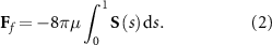
where u and p are the velocity and pressure fields of a fluid, respectively, and µ the dynamic viscosity. Considering a slender body of unit length, let ![${\mathbf{S}}\left( s \right) = {\left[ {{S_\parallel }\left( s \right),{S_ \bot }\left( s \right)} \right]^{\text{T}}}$](https://content.cld.iop.org/journals/1748-3190/18/3/035003/revision4/bbacbe86ieqn1.gif) be the distribution of Stokeslets [58], where the superscript T denotes transpose and 0 ⩽ s ⩽ 1 is the arclength along the body centerline. Applying the linear superposition method (equation (1a,b
) are linear) to solve the fluid field and pressure distribution, the total fluid force F
f
acting on a flagellum of unit length can be obtained as:
be the distribution of Stokeslets [58], where the superscript T denotes transpose and 0 ⩽ s ⩽ 1 is the arclength along the body centerline. Applying the linear superposition method (equation (1a,b
) are linear) to solve the fluid field and pressure distribution, the total fluid force F
f
acting on a flagellum of unit length can be obtained as:
Let P(s) and κ(s) be the coordinates and the half-width of the body at the position s along the body centerline, where κ(s) also indicates how slender the body is. If κ is sufficiently small and the cross-section is circular, one can obtain the classical expression of S based on the SBT [35]:
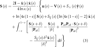
where  and
and  are orthogonal unit vectors that are tangential and normal to the body centerline, respectively, I the identity matrix, P
sδ
= P(s) – P(s + δ) the distance vector, and V(s) the local translational velocity of the body.
are orthogonal unit vectors that are tangential and normal to the body centerline, respectively, I the identity matrix, P
sδ
= P(s) – P(s + δ) the distance vector, and V(s) the local translational velocity of the body.
To deal with arbitrary flagellum cross-sections or 2D problems (i.e. with rectangular cross-sections), we follow the method proposed in [55] to introduce a dimensionless coefficient tensor K to the expression of fluid velocity field. Based on the SBT for circular flagellum cross-section, the relative fluid velocity field can be expressed as:  , where U(s) = u(s) – V(s) represents the relative velocity of the fluid with respect to the flagellum part at point s. For non-circular ones, it is assumed that the relative fluid velocity for the non-circular case is:
 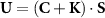 , where C is the resistive tensor, and the Stokeslets S is still based on the expression for a slender body with a circular cross-section. Note that the revised expression of U can still meet the zero-divergence condition for fluid velocity (i.e. equation (1b)) as long as K is a symmetric tensor with zero divergence.
In [55], K depends only on the shape of the cross-section, which can be directly estimated for some special shapes without performing FSI simulations. Nevertheless, in most cases, FSI simulations are required to determine K because the dynamics of a solid body (e.g. the wiggling profile of a flagellum), which affects U and K, cannot be determined a priori, as reported by Borker and Koch [56]. Hence, we assume that K = [Kij ] (i, j = 1, 2 for 2D problems) is the only correction tensor to determine and that it must be determined based on the comparison between FSI simulation and the SBT model. In the following, we reduce the corrected SBT to the corrected RFT by neglecting interactions between different parts of a flagellum. This is generally an acceptable simplification in the study of micro-swimmers [35] considering the limited accuracy in experimental observation. In RFT, the fluid forces F f acting on a slender body is assumed to be proportional to the local velocity of the body. We shall then include K in the coefficients of proportionality to establish the CRFT.
For shorthand, we recast equation (3) as:

where ![${\boldsymbol{\mit\kappa }}\left( s \right) = {{\left[ {2{\mathbf{I}} - {\hat{\mathbf{x}}}\left( s \right){\hat{\mathbf{x}}}\left( s \right)} \right]} \mathord{\left/ \right. } {\left[ {4\ln \kappa \left( s \right)} \right]}}$](https://content.cld.iop.org/journals/1748-3190/18/3/035003/revision4/bbacbe86ieqn6.gif) , and ψ[S(s)] is the functional of Stokeslets S(s) and ψ(0) = 0. Taking the correction term
, and ψ[S(s)] is the functional of Stokeslets S(s) and ψ(0) = 0. Taking the correction term  into account, equation (4) is rewritten as:

The approximation of equation (5) can be made based on the scenario of a straight flagellum of a uniform cross-section. In this scenario, U and κ are constants, and the direction vectors  and
and  are independent of position s, which greatly simplifies the solution. An iterative procedure can then be adopted. First, the zeroth-order approximation S(0)(s) can be determined by applying S = 0 to the right-hand side of equation (5) and is expressed as:

Substituting equation (6) into the right-hand side of equation (5) again results in the first-order approximation S(1)(s). The second-order approximation S(2)(s) can be obtained similarly and is normally accurate enough for the RFT [35]. Eventually, we can obtain the total fluid force F f on a uniform straight flagellum of unit length with a unidirectional motion by substituting S(2)(s) into equation (2).
Denoted by  and
and  the components of U(s) tangential and normal to the local centerline of a flagellum, respectively, the corresponding fluid forces in the RFT are formulated as:

Based on the second-order approximation S(2)(s) and equation (2), the two coefficients of resistive forces in equation (7a, b
) in the CRFT can be derived (cf appendix
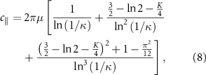
and
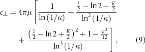
where the correction factor K = K11 = −K22 due to the property of zero divergence of the tensor K. Note that when K = 0, equations (8) and (9) reduce to the RFT expressions in [35]. The proposed CRFT is then applicable to formulate the governing equations of an AFMS based on the bar-joint model.
2.2. The bar-joint model
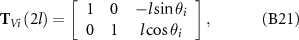
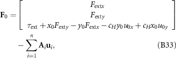
Figure 2 demonstrates the bar-joint model of the AFMS. The flagellum is simplified into rigid bars with a constant length 2 l. They are indexed (denoted by i) from 1 to n and connected with linear torsion springs [47]. The ith spring joint connects the bars i and (i+ 1) and the first (i = 1) bar is assumed to be rigidly connected to the head. The motion of the ith bar and the head (i = 0) can be represented by the vector of time-dependent variables X
i
(t) = (xi, yi, θi
)T, where xi
and yi
are coordinates of the midpoint of the ith bar (or the center of the head), and θi
the angle of rotation with respect to the x-axis (anticlockwise rotation is taken as positive). Correspondingly, the velocity vector of the head (i = 0) and bars (i > 0) can be represented by 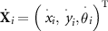 , where the overhead dot denotes time derivative.
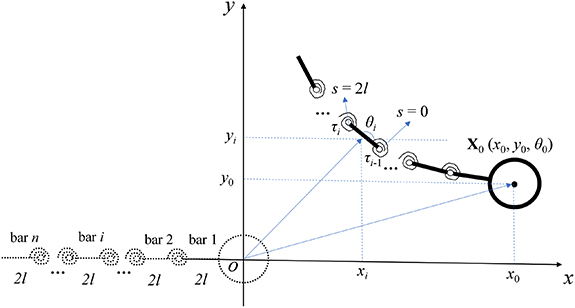
Figure 2. The schematic of the bar-joint model of the AFMS, where the global coordinate system is established with the origin at the centroid of the head and the x- and y-axes being the longitudinal and transverse axes of the flagellum at the initial state, respectively.
Download figure:
Standard image High-resolution imageBased on the CRFT, one can easily obtain the three equilibrium equations of external forces for the bar-joint model, given by:
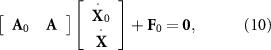
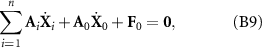
where A0
and A are the resistive matrices of the head and bars (detailed expressions can be seen in equations (B16) and (B19) in appendix
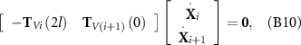
At the ith joint, the velocities determined from the two connected bars should be equal, i.e. V i (2l) = V i +1(0). These constraints ensure the inextensibility conditions of a flexible flagellum [48, 49]. Since the first bar and the head are assumed to be rigidly connected, one can obtain below (2n + 1) equations in terms of the constraints:
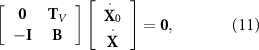
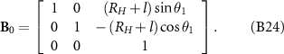
where I is a 3 × 3 identity matrix, T V the matrix of kinematic constraints of neighboring bars (see equation (B20)), and B the kinematic constraints between the first bar and the head (see equation (B23)).
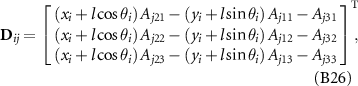
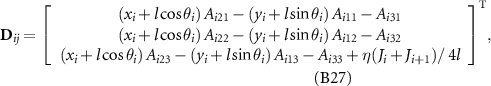
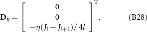
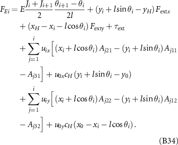
The polymeric (viscoelastic) flagellum is described based on the discrete beam theory [50] in which the inherent damping in most polymers is nonnegligible [24]. The material of the micro-swimmer is considered to be a kind of isotropic polymer described by the Kelvin–Voigt viscoelastic model [59]. The moment induced by the torsion spring at the ith joint Mi is expressed in a forward difference formula as:
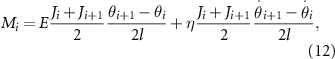
where E and η are the Young's modulus and viscosity coefficient, respectively [60–62], and Ji
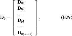
denotes the second moment of area of the ith bar, where an average value of J between two neighboring bars is adopted to indicate the second moment of area at the ith joint in case the flagellum is non-uniform. Then, the moment equilibrium of the structure leads to the below (n − 1) equations (cf appendix
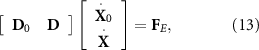
where D and D0 are the matrix of moment balance related to the bars and head, respectively, which are expressed in equations (B25) and (B29), and F
E
is a list of torques, which is expressed in equation (B31) in appendix
Finally, combining equations (10)–(13), the governing ODEs of the bar-joint model based on the CRFT can be expressed as:
The nondimensionalization of equation (14) can be taken by choosing the half-length of a bar l, the period of the acoustic actuation T = 1/fr
, and the fluid viscosity μ as the reference variables based on the Buckingham π theorem [63]. The dimensionless quantities are detailed in appendix
3. Results and discussion
3.1. Problem statement and convergence analyses of FSI simulations
We consider an AFMS requiring acoustic excitations to propel. The concerned AFMS is composed of a rigid head and a flexible slender flagellum, as exhibited in figure 3, where the structure has been meshed for the FSI simulation. The AFMS suspends in an aqueous solution and swims under an acoustic actuation that leads to the oscillations of the head and the whipping of the flagellum. According to the study of Liu and Ruan [24], the effect of periodic acoustic excitation for an AFMS can be assumed to be a periodic force Fext acting on the head with the actuation frequency fr
, that is  , where ω= 2πfr is the angular frequency and Fa
is the amplitude. The head oscillation induced by Fext whips the flagellum, giving rise to the advancement of the AFMS at an average speed of Vave. We focus firstly on the swimming problem that the average displacement of the micro-swimmer during several actuation periods keeps a straight line. It has been demonstrated both experimentally [14, 65] and theoretically [24, 40, 47] that the micro-swimmer tends to align itself perpendicular to the direction of Fext. Hence, in the following FSI simulations, the only boundary condition is that the centroid of the head (or the end of the flagellum if the micro-swimmer has no head) is subject to a transverse harmonic force Fext. Consequently, the head oscillates transversely with an amplitude Aamp.
, where ω= 2πfr is the angular frequency and Fa
is the amplitude. The head oscillation induced by Fext whips the flagellum, giving rise to the advancement of the AFMS at an average speed of Vave. We focus firstly on the swimming problem that the average displacement of the micro-swimmer during several actuation periods keeps a straight line. It has been demonstrated both experimentally [14, 65] and theoretically [24, 40, 47] that the micro-swimmer tends to align itself perpendicular to the direction of Fext. Hence, in the following FSI simulations, the only boundary condition is that the centroid of the head (or the end of the flagellum if the micro-swimmer has no head) is subject to a transverse harmonic force Fext. Consequently, the head oscillates transversely with an amplitude Aamp.
Figure 3. The configuration of a FSI simulation, wherein the gray area represents a mesh result of the fluid, and the blue area illustrates the deformable AFMS domain.
Download figure:
Standard image High-resolution imageFigure 3 shows the mesh of the FSI model that was simulated using a built-in fully coupled 2D FSI solver in COMSOL Multiphysics [66]. The whole geometry can be divided into two domains: a rectangular fluid domain of 2000 × 500 µm2 (capacious enough for a micro-swimmer) and a solid one for the AFMS in the center of the fluid. The radius of the circular head and the length of the flagellum are denoted by RH and L, respectively. For a 2D simulation, the cross-section of the flagellum is rectangular. The flagellar width Wy can be either uniform or tapered with a maximum of Wy 0 at the root (the joint between the head and the flagellum). The micro-swimmer is assumed to have a uniform thickness of Wz .
We investigate the steady-state swimming performances using the trajectory of the center of the head (or the right end of the flagellum). In the numerical simulations, the incompressible creeping flow module without the inertial term (Stokes flow) is employed for the fluid domain, while the solid mechanics module with plane strain approximation for the solid domain [67]. The micro-swimmer consists of two material models: a viscoelastic material for the flagellum and a rigid domain for the head [59]. Considering the expected medical applications and the current experiments, the flagellar material is assumed to be a Kelvin–Voigt viscoelastic material for representing an organic polymer, such as the polypyrrole employed in [13] and the polyethylene glycol employed in [14]. Fext is applied along the y-direction to the centroid of the head. If headless, Fext is applied to the right end of the flagellum. The automatic remeshing technique is employed to tackle the problems induced by large rigid-body motions, where the fluid domain (i.e. the gray area in figure 3) is set as the moving mesh region based on the Winslow smoothing method [68], in which the mesh distortion parameter is set to unity.
We first exemplify 2D simulations of two AFMS models as shown in figures 4(a) and (b). The first (figure 4(a)) one is a uniform flagellum (without head) with dimensions: L = 200 μm, Wz = 40 µm, and Wy = 12 µm, and swims in a fluid with the dynamic viscosity: µ = 0.1 Pa·s. The second one (figure 4(b)) is a sperm-like micro-swimmer referring to the AFMS described in [14]. It has a thickness, Wz = 20 µm, and a cylindrical head with a radius: RH = 20 µm, and a tapered flagellum: L = 200 μm and Wy = Wy 0(1 – λX), where 0 ⩽ X⩽ 1 is the length normalized by L, Wy 0 = 20 μm, and the tapering index λ = 0.9. Both micro-swimmers have the material properties: E = 10 MPa and η = 10 Pa·s and in the static fluids (u = 0).
Figure 4. Examples of convergence analyses of the FSI simulation with common parameters L = 200 μm, E = 10 MPa, η = 10 Pa s, µ = 0.1 Pa·s, Aamp = 20 μm, and fr = 1000 Hz: (a) the pressure distribution of a uniform flagellum without head at the end of the fifth actuation period (t = 0.005 s) with RH = 0, λ = 0, Wy 0 = 12 µm, Wz = 40 µm, and Fa = 2.7 µN; (b) the pressure distribution of a tapered flagellum with head at the end of the fifth actuation period (t = 0.005 s) with RH = 20 μm, λ = 0.9, Wy 0 = 20 µm, Wz = 20 µm, and Fa = 4 µN; (c) convergence analyses in terms of the number of elements for the cases with (red solid line) and without (blue dotted line) head.
Download figure:
Standard image High-resolution imageFigures 4(a) and (b) illustrate the fluid pressure distribution at t = 0.005 s. An vertical acoustic force Fext was applied at the right with a frequency of fr = 1000 Hz and an amplitude of 2.7 μN and 4 µN, for the uniform flagellum (figure 4(a)) and the sperm-like micro-swimmer (figure 4(b)), respectively, to maintain an amplitude of Aamp = 20 μm at the actuated end. It is observed that the average trajectory within a period of acoustic excitation is nearly a straight line parallel to the x-axis. The average (over one period) velocity in the first two periods varies (transient motion) and afterwards stabilizes at 383.4 μm·s−1 (figure 4(a)) or 5537 μm·s−1 (figure 4(b)). For the micro-swimmer herein, considering the fluid density ρ ∼ 103 kg·m−3, which leads to the Reynolds number Re = ρLV/μ = 7.668 × 10⁻⁴, which is sufficiently small to warrant the employment of the RFT. The stabilized terminal velocity Vave is obtained with the simulation domain having around 104 elements (figure 4(a)) or 2 × 10⁴ elements (figure 4(b)). Figure 4(c) illustrates the relative errors for the cases without and with head, respectively, in terms of the number of elements used in the FSI simulations. It is noted that the simulation results have converged (i.e. the deviation is within 5%) when the number of elements is more than 104, indicating that the FSI simulation is convergent and stable.
3.2. Determination of K
The correction factor K is determined by comparing the terminal average velocities Vave obtained from the FSI simulations and the CRFT-based bar-joint model (the convergence analysis of the bar-joint model can be seen in appendix
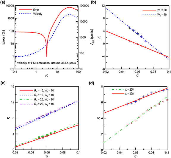
Figure 5. Estimate of K for uniform flagella with parameters η = 10 Pa·s, µ = 0.1 Pa·s, and Aamp = 20 μm (other paramours are provided in table 1): (a) example of the error (red solid line) Vave obtained from the CRFT model (blue dashed line) based on the simulation result (Vave = 383.4 μm·s−1) when K varies; (b) relations between K and α for a flagellum without head; (c) relations between K and α for an AFMS with head; (d) relations between K and α for AFMSs with different flagellum length.
Download figure:
Standard image High-resolution imageTable 1. The fitting expressions of K in terms of α, λ or β under different combinations of geometric parameters.
| L (μm) | RH (μm) | Wz (μm) | Wy 0 (μm) | λ | fr (Hz) | E (MPa) | Μ (μm) | Expression of K | Figures |
|---|---|---|---|---|---|---|---|---|---|
| 200 | 0 | 20 | 10–14 | 0 | 1000 | 10 | 0.1 | K = −104α + 6.08 | 4(b) |
| 200 | 0 | 40 | 10–14 | 0 | 1000 | 10 | 0.1 | K = −204α + 15.32 | 4(b) |
| 200 | 10 | 20 | 10–14 | 0 | 1000 | 10 | 0.1 | K = 7α – 0.72 | 4(c) |
| 200 | 10 | 40 | 10–14 | 0 | 1000 | 10 | 0.1 | K = 90α + 3.32 | 4(c) |
| 200 | 20 | 20 | 10–14 | 0 | 1000 | 10 | 0.1 | K = 72α – 0.5 | 4(c) |
| 200 | 20 | 40 | 10–14 | 0 | 1000 | 10 | 0.1 | K = 86α + 3.84 | 4(c) |
| 400 | 20 | 20 | 20–40 | 0 | 1000 | 10 | 0.1 | K = 39.27α + 3.854 | 4(d) |
| 200 | 20 | 20 | 20 | 0.1–0.9 | 1000 | 10 | 0.1 | K = −1.29λ + 6.43 | 5(a) |
| 200 | 20 | 20 | 20 | 0.9 | 500–7000 | 10 | 0.1 | K = (0.036β2 + 2.40β+ 24.5)/(β + 0.12) | 5(b) |
| 200 | 20 | 20 | 20 | 0.9 | 1000 | 3–70 | 0.1 | K = (0.087β2 – 2.07β+ 106)/(β + 7.78) | 5(b) |
| 200 | 20 | 20 | 20 | 0.9 | 1000 | 10 | 0.05–0.7 | K = (0.016β2 + 1.40β+ 41.4)/(β + 0.89) | 5(b) |
In principle, adjusting K can lead to an excellent agreement between simulation and CRFT results. In the following estimate of K for different cases, we set the criterion of acceptable deviation in Vave to be 5% to balance the computational efficiency and accuracy and demonstrate several relations between K and the flagellum slenderness α (α = Wy /L) in figures 5(b)–(d). In order to ensure that the flagellum is still a slender body, we set α in the range of 0.05–0.07 [31]. Figures 5(b) and (c) show that K varies almost linearly with α, and the slope depends on the thickness Wz, for both the uniform flagellum without a head and the sperm-like micro-swimmer with a rigid-cylindrical head, respectively. The detailed expressions of K in terms of α obtained through linear regression are listed in table 1.
In table 1, one can note that the existence of a head can change the slope of the linear K–α relation from a negative value to a positive one. Besides, as observed in figure 5(c), the variation of RH can hardly influence the K–α curve. In addition, K doubles when the depth Wz increases from 20 to 40 µm, as shown in figures 5(b) and (c), and also doubles when L increases from 200 to 400 µm, as shown in figure 5(d). These results suggest that, roughly speaking, K is linearly dependent on the volume of the flagellum. In figure 5(d), α is sampled from 0.05 to 0.1, and the fitting equation obtained in the α range of 0.05–0.07 is used. In the 0.07–0.1 range, the difference between the fitting equation and the actual results of K are still below 3%.
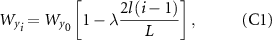
When a tapered flagellum is discretized into be a bar-joint model, these bars have uniform dimensions. In this case, the fitting equations of K for a uniform flagellum may be directly employed. For example, consider the micro-swimmer with L = 200 µm and RH = Wz = Wy 0 = 20 µm, assume that the width of the ith bar, i.e. Wyi , follows the tapering equation (equation (C1)) and that the slenderness of the ith bar, i.e. αi , equals Wyi /L, the correction factor of the ith bar, i.e. Ki , can then be estimated according to the fitting curve of K in figure 5(d). In this way we can directly obtain the terminal average velocity Vave based on the CRFT model without implementing the FSI simulation. We herein designate this method as the direct-K method. Straightforward though this method is, its outcomes can deviate from those of the FSI simulation, and the corresponding error in terms of the tapering index λ is illustrated in blue dotted line in figure 6(a). For the classical RFT model, i.e. Ki = 0 for each bar, the error exceeds 90%. For the direct-K method, it is noted that the error is around 12% for λ > 0.2, which indicates that if we directly apply the fitting expression of K arising from the case of a uniform flagellum to the case of a tapered one, the error can decrease by about 80% from the results of RFT. However, the deviation is still considerable.
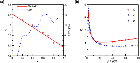
Figure 6. Estimate of K for tapered flagella with parameters η = 10 Pa·s, µ = 0.1 Pa·s, and Aamp = 20 μm (other paramours are provided in table 1): (a) relations between K and λ and between the error and λ, respectively, where the fitting curve of K (red solid line) is obtained by the effective-K method, and the error of Vave (blue dotted line) is obtained by the direct-K method; (b) the relation between K and β obtained by varying fr (red cross), E (blue circle), or μ (blue star), respectively.
Download figure:
Standard image High-resolution imageMore accurate results for a tapered flagellum can be achieved by assuming all bars having identical K, i.e. Ki = K. In this way, we treat a tapered flagellum to be an equivalent uniform one with an effective K, and thus this method is regarded as the effective-K method. The red circles in figure 6(a) represent the effective K at different λ, and the red solid line is the corresponding linear fitting: K = −1.29λ + 6.43. It is noted that in figure 6(a) for λ ⩽ 0.1, magnitude of the effective K is nearly identical to that of the case of λ = 0, and the error of the effective-K method is close to 0, indicating that the effect of tapering on hydrodynamics only works when λ > 0.1.
Note that the above results of K are obtained with the specific material and actuation parameters. We find that Aamp and η hardly affect the determination of K, while fr, E and μ can have considerable influence. For example, for the micro-swimmer as shown in figure 4(b) in section 3.1, we varied fr, E and μ to check their influence on K. It is noted that the combined term β = μfr
/E is an important non-dimensional parameter in the governing equations of flagellum's hydrodynamics. For example, β enters into the elastohydrodynamic penetration length [40]: ![$\sqrt[4]{{\left( {EJ} \right)/\left( {2\pi {c_ \bot }{f_r}} \right)}}$](https://content.cld.iop.org/journals/1748-3190/18/3/035003/revision4/bbacbe86ieqn14.gif) , proportional to
, proportional to![$\sqrt[4]{{{1 \mathord{\left/ \right. } \beta }}}$](https://content.cld.iop.org/journals/1748-3190/18/3/035003/revision4/bbacbe86ieqn15.gif) , and the sperm number [69]:
, and the sperm number [69]: ![$L\sqrt[4]{{\left( {2\pi {c_ \bot }{f_r}} \right)/\left( {EJ} \right)}}$](https://content.cld.iop.org/journals/1748-3190/18/3/035003/revision4/bbacbe86ieqn16.gif) , proportional to
, proportional to ![$\sqrt[4]{\beta }$](https://content.cld.iop.org/journals/1748-3190/18/3/035003/revision4/bbacbe86ieqn17.gif) . Hence, we plot the relations between K and β in figure 6(b) with the corresponding fitting equations listed in table 1. It is noted that when β is between 5 and 20, the variations of K in terms of fr, E and μ collapse to the same curve. When β >20, the effects of E and μ are still the same and tends to level off; nevertheless, the effect of head excitation frequency fr
tends to lean upwards. The difference in K increases with the increase in fr
and μ (or decrease in E) when β> 20 because raising fr
can considerably enhance Vave (which leads to a larger K) as it can induce the change of the flagellum's wiggling profile (e.g. bringing about smaller wavelength). Instead, increasing μ or reducing E only leads to larger resistive forces under the same wiggling profile, which results in a small enhancement in Vave.
. Hence, we plot the relations between K and β in figure 6(b) with the corresponding fitting equations listed in table 1. It is noted that when β is between 5 and 20, the variations of K in terms of fr, E and μ collapse to the same curve. When β >20, the effects of E and μ are still the same and tends to level off; nevertheless, the effect of head excitation frequency fr
tends to lean upwards. The difference in K increases with the increase in fr
and μ (or decrease in E) when β> 20 because raising fr
can considerably enhance Vave (which leads to a larger K) as it can induce the change of the flagellum's wiggling profile (e.g. bringing about smaller wavelength). Instead, increasing μ or reducing E only leads to larger resistive forces under the same wiggling profile, which results in a small enhancement in Vave.
3.3. Examples of verification
In order to explicate the validity of the method for correcting RFT, we compare three head trajectories (or the trajectories of the right end of the flagellum for the case without head) calculated by FSI simulations and by CRFT. Figure 7 exhibits the trajectories and their errors from FSI simulations and the CRFT models for the acoustic-actuation period from 20 to 25. The corresponding geometries of AFMSs at four instances which equally divide the last period in the FSI simulation (outline) and the CRFT model (centerline) are given as the insets. The supplementary videos of the corresponding FSI simulations and relevant codes of the CRFT model for verification are provided in the supplementary documents.

Figure 7. Verifications of the CRFT model: the head trajectories obtained from the FSI simulations (red lines) and CRFT-based bar-joint models (blue lines) for the cases of (a) a uniform flagellum without head, (c) a uniform flagellum with head, and (e) a tapered flagellum with head, and (b) and (d) and (f) the corresponding trajectory errors which are the distances between two head positions at the same time scaled by the length of the flagellum, respectively. The marked points in (b) and (d) and (f) indicate that the trajectory errors reach their extreme values, where the corresponding distances between the pairs of trajectory points are indicated by the dashed lines in (a) and (c) and (e). To have a clearer comparison, only the periods from 20 to 25 are shown. The insets in (b) and (d) and (f) show the trajectory errors for a long time (40 periods).
Download figure:
Standard image High-resolution imageFigures 7(a), (c) and (e) show the trajectories of FSI simulations and CRFT models for the case of a uniform flagellum without a head, a uniform flagellum with a head, and a tapered flagellum with a head, respectively. To approximate the trajectories based on the CRFT model, the corresponding K are determined to be 3.2, 6.3, and 5.2, respectively, based on the fitting equations suggested in the last section. It is noted that each of the trajectories obtained based on the CRFT model has an offset from the FSI-simulated one, reflecting the slight difference in the propulsive forces. This is due to the determination of K, in which we allowed a 5% tolerance in the motility difference. The distance between the positions of the AFMS head obtained from the FSI simulation and those from the CRFT solution, after dividing by the flagellum length L, is defined as the position error of CRFT solution, which are shown in figures 7(b), (d) and (f) (from 20 to 25 periods) and their insets (for first 40 periods). One may note that in figures 7(b) and (f), there are some small spikes, whereas in figure 7(d) the errors are simply oscillating. Several extreme error points in figures 7(b), (d) and (f) are indicated in figures 7(a), (c) and (e), respectively, where the corresponding differences between the two solutions are indicated by dashed lines. It is noted that the spikes of errors are due to the oscillatory motions, resembling the interference of waves.
The insets in figures 7(b), (d), and (f) show that the position errors in 40 periods are well below 4%. Because of the small motility difference (i.e. the tolerance in determining K), the trajectory deviations are caused; nevertheless, these deviations are well bounded and remain small when normalized by the length of the flagellum. Such small errors indicate that the CRFT-based bar-joint model, as described in section 3, renders an excellent approximation to numerical simulations. It should be noted that such position errors can be further reduced if we set a more stringent requirement in accuracy in determining K.
3.4. An application of the CRFT-based bar-joint model
We expect that the proposed CRFT-based bar-joint model can ultimately be employed for the path planning and navigation control of AFMSs because of the excellent agreement between the FSI and the simplified model has been revealed. Here, as the final demonstration, we employ CRFT to study the turning strategy for an AFMS, which is essential and inevitable in practical applications. It is noted that FSI simulation for turning is unconverted in our trials due to excessively distorted elements; hence, we only provide the results of CRFT model.
In the following demonstration, the AFMS is identical to the one shown in figure 7(e). We expect that the external force Fext (Fext = [Fextx , Fexty ]T) can be applied to the head of an AFMS through applying acoustic waves. According to [24], under an acoustic planewave rendering a 2D fluid displacement field Aacou with the amplitude Aacou, the oscillation amplitude of the head (RH = 20 μm) of the AFMS Aamp is approximately 1.67Aacou if the sound wavelength is far greater than the dimensions of the head. In this case, the oscillatory velocity in the fluid is nonzero, i.e. u = ∂Aacou/∂t.
One may note from the trajectories in figure 7 that an AFMS tends to move along the direction perpendicular to Fext that induces head oscillations, which is also the case in the experiments of acoustic actuation [65]. Hence, steering an acoustically propelled AFMS might be achieved by rotating Fext and we can design such a turning method using only acoustic power based on the CRFT model. Considering an acoustic planewave that can gradually change the direction of propagation, hence changing the direction of Fext on the head of an AFMS. As shown in figure 8(a), we let the angle of the acoustic wavevector rotates from 90° to 60° (counterclockwise from positive direction of x-axis) in 10 periods. After the change, the angle of the micro-swimmer is around 5°. Maintaining Fext at 60° for 100 periods, the angle of the AFMS gradually drift to be close to 60°. Further turning Fext to 150° in 10 periods leads the angle of the micro-swimmer to move along the straight line of 60°. The detailed trajectory of the AFMS is shown in figure 8(b).

Figure 8. Application of the CRFT model where the AFMS is steered by acoustic waves: (a) the rotation angle with respect to the x-axis in terms of actuation period for the acoustic waves (blue dashed line) and the AFMS (red solid line); (b) the trajectory and orientations of the AFMS within 150 periods; the insets sketch the acoustic steering strategy, and the time t is in terms of the number of acoustic periods.
Download figure:
Standard image High-resolution imageThe above example shows that using only acoustic power to control AFMSs is possible in theory, although the orientation relation between an AFMS and acoustic wavevector is nontrivial, depending on the parameters of the actuation and the swimmer [70]. If the direction of wavevectors can be accurately adjusted, these waves can induce head oscillation and flagellum wiggling for propulsion and steering. In these attempts, our AFMS model can provide the formalism for the trajectory prediction and manipulation, which will lay the foundation for controlling micro-swimmers to carry out precision therapies for cancers and other diseases requiring non-invasive and localized treatments.
If a torque can be applied to the head of an AFMS, turning will be easier and more controllable. This can be achieved by introducing magnetic particles (MPs) into the head [71], resulting in a magnetized head along an easy axis (M), and applying an external magnetic field (B) unparallel with the head's easy axis, resulting in a torque τext = M× B on the head, as sketched in the inset in figure 9(b). Note that the acoustic power is still used for propulsion but not for steering. The external magnetic field used in hyperthermia-based therapy is usually around 10 mT [72] and that the volumetric magnetic susceptibility is in the order of 105 for ferromagnetic MPs [73], accordingly, the magnetic-induced torque by single MP of 1 μm is around 4 × 10⁻¹² N·m. With five MPs in the head, the total magnetic torque on the head is 2 × 10⁻¹¹ N·m, which is assumed in the following calculation. For such a magneto-acoustic method, we design the variations of Fextx , Fexty and τext as shown in figure 9(a), which results in the trajectory of the AFMS as shown in figure 9(b). Hence, the proposed magneto-acoustic maneuver is feasible based on the existing technologies and our theoretical analysis of magneto-acoustic steering can be employed for targeted therapies which require the accurate and rapid navigation.
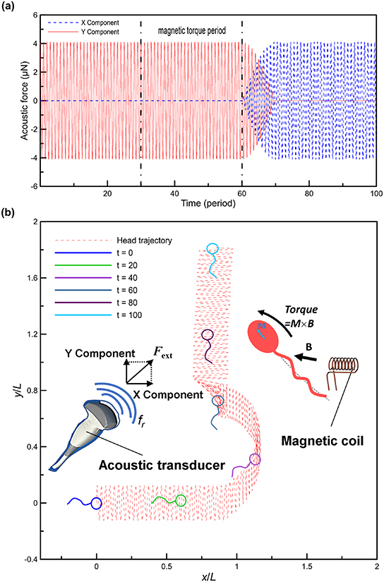
Figure 9. Application of the CRFT model where the AFMS is steered by a magneto-acoustic strategy: (a) the applied acoustic forces for propulsion in terms of actuation period along x (blue dashed line) and y (red solid line) directions (Note: the actuation forces along y (x) direction linearly decreases (increases) between the 60th period and the 70th period to assist turning), and from the 30th and 60th periods, a magnetic torque is applied; (b) the trajectory and orientations of the AFMS within 100 periods; the insets sketch the remote magneto-acoustic steering strategy.
Download figure:
Standard image High-resolution image4. Conclusions
In this work, we have described a CRFT and the CRFT-based 2D bar-joint model for modeling AFMSs propelled by acoustic actuation. The main purpose of this work is to allow a simplified AFMS model to be correctable, verifiable, and in future, applicable for practical applications. The CRFT is inspired by the derivation of the SBT for non-circular flagellum and only introduced is the single correction factor K. However, K depends on not only geometrical parameters but also other factors influencing a flagellum's wiggling profiles, such as material properties and actuation frequency. Hence, although the CRFT is derived from the non-circular SBT, K should be determined after some knowledge of the motility of an AFMS are obtained. In the exercises, we determined K by comparing the terminal average velocities obtained from the CRFT-based bar-joint models propelled by acoustic waves and those from the FSI simulations. After correction, it is shown that the difference in the detailed trajectory can be well below 4%. In our work, K is very weakly dependent on the head radius RH and linearly dependent on the slenderness α and the tapering factor λ. Hence, it is not difficult to determine these dependences and then employ CRFT to optimize the geometry of an AFMS for maximizing the motility. With CRFT, the controlled navigation of AFMSs can also have a high-level robustness. For this point, we have demonstrated the possible strategies of turning an AFMS using acoustic or magneto-acoustic fields, which indicates that the current CRFT model includes enough information to deal with a turning activity.
Before closing this work, the insufficiency of the current CRFT model must be remarked. The current empirical method for the determination of K is tedious and ungeneralizable to the scenarios beyond the parametric space studied in this work, as it requires FSI simulations. An analytical expression of K as a function of geometric, materials, and actuation parameters of an AFMS (i.e. without simulation) is desired, which will be our effort in the future work. In addition, the effectiveness of the CRFT model has not been examined in experiments. It is necessary to fabricate AFMS embedded with magnetic nanoparticles to determine the motility and magneto-acoustics turning performance to verify our model. As the final remark, we stress that this work only analyzed the propulsion caused by oscillations of the head of a microswimmer. The effect of acoustic streaming on the tip of a flagellum, as discussed in [13, 74], was not analyzed. Such a tip force field may also induce the wiggling of a flagellum. In our model, it may also be simplified to be the external force, F0, acting on the tip. The detailed expression of such tip-induced propulsion is worth exploring in future work.
Acknowledgments
This work was supported mainly by NSFC/RGC Joint Research Scheme (Project No. N_PolyU519/19) and partially by the project of International Cooperation and Exchanges of NSFC (No. 51961160729). The authors are grateful for the financial support.
Data availability statement
All data that support the findings of this study are included within the article (and any supplementary files).
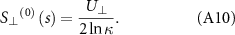
Appendix A: Detailed derivation of the CRFT
When a slender body with uniform cross-section remains straight in motion, U and κ become constants and the direction vectors  and
and  are independent of position s, i.e.
  , and
, and  . Hence, equation (5) can be simplified as:
When the body moves tangentially to its centerline, resulting in the Stokeslet vector  , and the relative velocity
  , then equation (A1) is recast as:
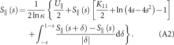
The zeroth iterative of equation (A2) is expressed as:
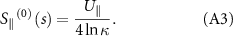
Replacing  on the right side of equation (A2) with the right-hand side of equation (A3) reaches the first iterative of the tangential Stokeslet, expressed as:
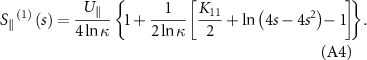
Replacing  on the right side of equation (A2) with the right-hand side of equation (A4) reaches the second iterative of the tangential Stokeslet, expressed as:
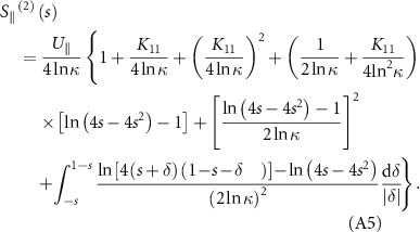
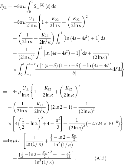
Then the total tangential fluid force of the slender body of unit length can be obtained based on equation (2) and is expressed as:
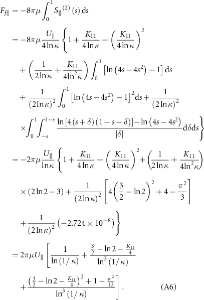
The tangential coefficient of resistive force, i.e. equation (8), can be obtained from equation (A6) by setting K11 = K (note we have assumed that K22 = −K11 due to the property of zero divergence of the tensor K). It is found that the influence of δ on the integral is negligible (∼10−8), which justifies RFT. To compare this expression with the classical one, we can construct the identical equation with non-zero constants x, a, and b, which is expressed as:
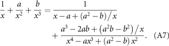
If x = ln(1/κ) is much larger than a and b, we can only keep the first term of the right side of equation (A7), and accordingly, equation (A6) will be simplified to
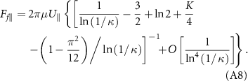
When K = 0, equation (A8) reduces to the classical RFT expression (cf equation (19) in [35]). However, in our work, ln(1/κ) is around 3, and K is uncertain. Therefore, the approximation of equation (A8) does not work; instead, equation (A6) should be used.
When the body moves perpendicularly to its centerline, resulting in the Stokeslet vector  , and the relative velocity
  , then equation (A1) is recast as
The zeroth iterative of equation (A9) is expressed as:
Replacing  on the right side of equation (A9) with the right-hand side of equation (A10) renders the first iterative of the normal Stokeslet, expressed as:
Replacing  on the right side of equation (A9) with the right-hand side of equation (A11) reaches the second iterative of the normal Stokeslet, expressed as:
Then the total fluid force normal to the slender body of unit length is expressed, based on equation (2), as:
The normal coefficient of resistive force, i.e. equation (9), can be obtained from equation (A13) by setting K22 = –K due to the zero divergence of K. Similarly, equation (A13) can also be simplified under the condition of sufficiently large ln(1/κ), which is expressed as:
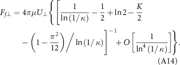
When K = 0, equation (A14) reduces the classical RFT expression (cf equation (20) in [35]). However, we use equation (A13) in our work because ln(1/κ) is not large, and K is uncertain.
Appendix B: Detailed derivation of the equations of motion based on the bar-joint model
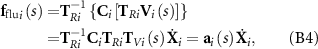
A point P in the ith bar with the distance s from the joint (i – 1) has the coordinate P i (s) expressed as:

Note that the coordinates of the head center P0 = (x0, y0)T is independent of s, which is be employed to track the trajectory of the micro-swimmer. Differentiating the right-hand side of equation (B1) with respect to time yields the translational velocity V i (s):
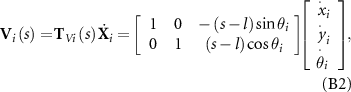
where T Vi (s) is the transformation matrix of velocity for the points in the ith bar.
To simplify the derivation, we first assume that the swimmer suspends in a static fluid field, i.e. u = 0. Hence, the relative velocity U = –V, and the total fluid forces on a rigid slender body, i.e. equation (7a,b
), are recast to  and
and  . Based on the RFT, the resistive coefficients
  and
and  are assumed to be constant even if the body is flexible and curved, i.e. the tangential and vertical components of local fluid forces f
f
(s) at position s can be formulated as:
are assumed to be constant even if the body is flexible and curved, i.e. the tangential and vertical components of local fluid forces f
f
(s) at position s can be formulated as: 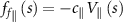 and
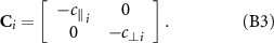
and  . Consequently, the tensor of resistive coefficients C
i
for the ith bar based on the CRFT can be expressed as:
. Consequently, the tensor of resistive coefficients C
i
for the ith bar based on the CRFT can be expressed as:
Note that C i varies with i because the bar width may vary when considering a tapered flagellum. The fluid forces fflui (s) at position s of the ith bar is then expressed as:
where ![${{\mathbf{T}}_{Ri}} = \left[ {\begin{array}{*{20}{c}} {\cos \theta {}_i}&{\sin {\theta _i}} \\ { - \sin {\theta _i}}&{\cos \theta {}_i} \end{array}} \right]$](https://content.cld.iop.org/journals/1748-3190/18/3/035003/revision4/bbacbe86ieqn36.gif) is the transformation matrix of rotation and the 2 × 3 resistive matrix a
i
(s) depends on the position s of the ith bar. We introduce the unit vectors e1 = (1, 0, 0)T, e2 = (0, 1, 0)T, and e3 = (0, 0, 1)T to facilitate derivations and the resultant fluid force vector Fflui
for the ith bar. The latter is given by:
is the transformation matrix of rotation and the 2 × 3 resistive matrix a
i
(s) depends on the position s of the ith bar. We introduce the unit vectors e1 = (1, 0, 0)T, e2 = (0, 1, 0)T, and e3 = (0, 0, 1)T to facilitate derivations and the resultant fluid force vector Fflui
for the ith bar. The latter is given by:
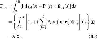
where the operators × and ⊗ indicate cross and outer products of two vectors, respectively, the 3 × 3 tensor A
i
is the fluid resistive matrix of the ith bar, and the augmented identity matrix ![${{\mathbf{I}}_a} = {\left[ {\begin{array}{*{20}{c}} 1&0&0 \\ 0&1&0 \end{array}} \right]^{\text{T}}}$](https://content.cld.iop.org/journals/1748-3190/18/3/035003/revision4/bbacbe86ieqn37.gif) is employed to extend the number of rows from 2 to 3 (note that the third component of Ffuli
is the resultant torque about the origin of the coordinate system due to fluid forces). We assume that the hydrodynamic resultant forces and torque on the circular head Fflu0 can be expressed as:
is employed to extend the number of rows from 2 to 3 (note that the third component of Ffuli
is the resultant torque about the origin of the coordinate system due to fluid forces). We assume that the hydrodynamic resultant forces and torque on the circular head Fflu0 can be expressed as:
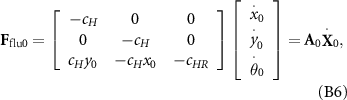
where cH and cHR are coefficients of resistance and are dependent on the head geometry and fluid viscosity [75]. Note that for a 2D FSI simulation, a circular head is a cylinder instead of a sphere. In this case, cH should be proportional to the thickness of Wz with a coefficient of resistance related to the Reynolds number, expressed as [76]:
where γ ≈ 0.577 is the Euler's constant, and the Reynolds number of the head Re = 2ρVRH /μ. For the micro-swimmer herein, considering the fluid density ∼103 kg·m−3, and the terminal velocity V ∼ 10−3 m·s−1, Re can be estimated to be 2RH /μ. The rotational drag coefficient of the head cHR is determined by [58]:

Then the equilibrium equations for the whole micro-swimmer can be given by
or equation (10).
At the ith joint, the velocities determined from the two connected bars should be equal, i.e. V i (2 l) = V i +1(0), which after substituting equation (B2), gives rise to the kinematic constraints:
where i runs from 1 to (n – 1). Since the first bar and the head are assumed to be rigidly connected, one can obtain the below ODEs in terms of the constraint:
For shorthand, equations (B10) and (B11) can be combined as equation (11).
For the moment equilibrium, as demonstrated in figure S1, torques are taken about the origin. The reaction forces at the ith joint FRx and FRy can be determined by the balance of forces over the first i bars and the head. The moment equilibrium of the structure before the ith joint leads to the below equations:
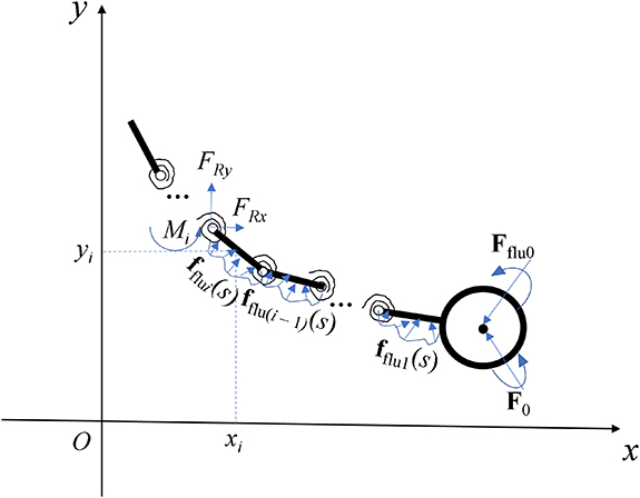
Figure S1. The diagram of force analysis for the bar-joint model.
Download figure:
Standard image High-resolution imagewhere i runs from 1 to (n – 1). Substituting equations (B3), (B4), (B9) and (12) into (B12) gives rise to the moment equilibrium of the structure, i.e. equation (13).
Finally, combining equations (10)–(13), the governing ODEs of the bar-joint model based on the CRFT can be expressed as equation (14). The equations of motion (equation (14)) are a set of (3n + 3) ODEs, in which the velocity vectors are:
where
and the velocity vector of head:
The 3 × 3 n resistive matrix of the flagellum is expressed as:

where
and the nine components of A i are respectively expressed as:
The resistive matrix of a head, as given in equation (B6), is expressed as:
The matrix of kinematic constraints of neighboring bars is expressed in the form of:
where
The 3 × 3n matrix B, obtained from the kinematic constraint between the first bar and the head, is expressed as:

where
The matrix of torque balance related to the joints D is expressed in the form as:
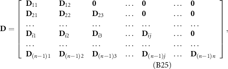
where i runs from 1 to (n – 1), and j from 1 to (i + 1). The expression of row vector D ij is dependent on the relation between i and j: when j < i, D ij is expressed as:
when j = i, D ij is expressed as:
when j = i + 1, D ij is expressed as:
The matrix of torque balance related to head is expressed as:
where the row vector D0i is expressed as:
The vector of velocity-independent torques is expressed as:
where the ith component FEi is expressed as:
When a micro-swimmer suspends in a non-static fluid circumstance, e.g. in a plane acoustic field with the velocity of fluid at the location of the ith bar u
i
= (uix, uiy
, 0)T (it is u0 at the head), then for the relative velocity U = u – V, the equations of local fluid forces will be recast as  and
and  . Eventually, the governing equations equation (14) will maintain the form except that the right-hand side non-homogenous terms must be revised to:
The Buckingham π theorem [63] is employed for nondimensionalization. We take the half-length of each bar l, the period of acoustic actuation T = 1/fr , and the fluid viscosity μ as repeating variables, then the following non-dimensional terms are introduced:
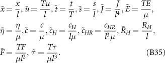
The dimensionless governing equations equation (14) can then be reached, where the three variables l, T, and μ become unity, and other physical quantities can be directly replaced according to equation (B35).
Appendix C: Convergence analyses of the bar-joint model
Here we show an example of the convergence analysis of the bar-joint model. For the convenience of comparisons, all the geometric and material parameters have the same values as those in the 1D classical continuum model reported in [24] in which the cross-section of the tapered flagellum is circular with the largest diameter Wy 0 = 25 μm and the tapering index λ = 0.9. Hence, for the bar-joint model, if we take the diameter at position P i (0) of a continuum flagellum as the diameter of the ith bar, i.e. Wyi , of a bar-joint flagellum, then Wyi can be derived given by:
where i is from 1 to n. The head is assumed to be a sphere with a radius of RH = 25 μm, and the effect of the spherical head on locomotion is accounted for by the coefficient of resistance cH given below as reported in [24],

Other parameters in the bar-joint model are: K = 0 (i.e. for the circular cross-section, the CRFT reduces to the RFT), cHR = 0 for eliminating the resistive effect of head rotation, u = 0, Fextx = 0, Fexty = Fa cosωt, τext = 0, fr = 4600 Hz, L = 180 μm, E = 10 MPa, η = 1730 Pa·s, µ = 1 Pa·s, and Fa = 344 µN to make Aamp = 20 μm.
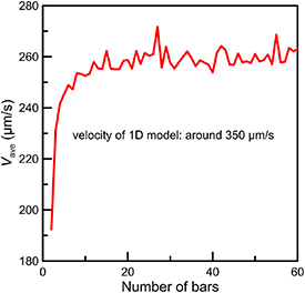
For the bar-joint model of the AFMS with a head (RH = 25 μm), we solve the governing ODEs, i.e. equation (14), by using the built-in solver ode15s in MATLAB [64]. The number of bars n varies from 2 to 60, and Vave is the position change of the head in the fifth period times fr . The result of Vave increase with n and levels off (with fluctuations) when n > 20, as illustrated in figure S2. Note that the analytical result in [24] is ∼350 μm·s−1 when Aamp = 20 μm. The converged result of the bar-joint model is ∼260 μm·s−1, 25% smaller from the analytical result in [24]. Such a deviation is in accordance with the expectation (see discussions in [31, 37]) because the 1D analytical model cannot involve the effect of rigid-body rotation which greatly affects the locomotion. Other factors, such as the ignorance of inextensibility and large deflection, also contribute substitutionally to the error of the 1D analytical model.
Figure S2. The convergence analysis of the bai-joint model in terms of the number of bars with parameters identical to results of figure 10(d) in [24], i.e. the terminal velocity is around 350 μm·s−1 when amplitude is 20 μm.
Download figure:
Standard image High-resolution image
Without the head (6.7 MB AVI)
Head and a constant flagellum (6.5 MB AVI)
Head and a tapered flagellum (6.3 MB AVI)
CRFT codes for verification (<0.1 MB ZIP)