
Abstract
Hippocampal reverse replay, a phenomenon in which recently active hippocampal cells reactivate in the reverse order, is thought to contribute to learning, particularly reinforcement learning (RL), in animals. Here, we present a novel computational model which exploits reverse replay to improve stability and performance on a homing task. The model takes inspiration from the hippocampal-striatal network, and learning occurs via a three-factor RL rule. To augment this model with hippocampal reverse replay, we derived a policy gradient learning rule that associates place-cell activity with responses in cells representing actions and a supervised learning rule of the same form, interpreting the replay activity as a 'target' frequency. We evaluated the model using a simulated robot spatial navigation task inspired by the Morris water maze. Results suggest that reverse replay can improve performance stability over multiple trials. Our model exploits reverse reply as an additional source for propagating information about desirable synaptic changes, reducing the requirements for long-time scales in eligibility traces combined with low learning rates. We conclude that reverse replay can positively contribute to RL, although less stable learning is possible in its absence. Analogously, we postulate that reverse replay may enhance RL in the mammalian hippocampal-striatal system rather than provide its core mechanism.
Export citation and abstract BibTeX RIS

Original content from this work may be used under the terms of the Creative Commons Attribution 4.0 license. Any further distribution of this work must maintain attribution to the author(s) and the title of the work, journal citation and DOI.
1. Introduction
Reinforcement learning (RL) is an area of machine learning where task learning takes place without explicit instructions; only generic feedback of success or failure (reward or punishment). This type of learning took inspiration from early behavioural studies in animals [57]. Due to its biological routes, there have been attempts to link RL back to animal behaviour (e.g. [32]), relate it to decision making (see [36] and references within), or explain RL within the context of neurobiology (e.g. [53, 54]).
Beyond this, many of the challenges in developing efficient and adaptable robots are RL problems; consequently, there has been no shortage of attempts to apply RL methods to robotics [30, 31, 57]. However, robotics also poses significant challenges for RL systems. These include continuous state and action spaces, real-time and end-to-end learning, reward signalling, behavioural traps, computational efficiency, limited training examples, non-episodic resetting, and lack of convergence due to non-stationary environments [31, 33, 67]. With continued developments in biology, particularly in neuroscience, it would be wise to continue transferring insights from biology into robotics [47] via RL techniques.
Yet equally important is its inverse, the use of our computational and robotic models to inform our understanding of biology [38, 63]. Robots offer a valuable real-world testing opportunity to validate computational neuroscience models [2, 4, 8, 28, 38, 45, 46, 55]. Therefore, our work falls in this medium between robotics and biology: we take inspiration from a phenomenon known as 'reverse replay' [12], in which recently active hippocampal cells reactivate in the reverse order to ask what potential advantages this phenomenon could bring RL. We then use these observations to inform biological hypotheses.
Though the neurobiology of RL has primarily centred on the role of dopamine as a reward prediction error signal [50, 54], there are still questions surrounding how brain regions might coordinate with dopamine release for effective learning. Behavioural timescales evolve over seconds, perhaps longer, whilst the timescales for synaptic plasticity in mechanisms such as spike-timing-dependent plasticity evolve over milliseconds [3]. How does the nervous system bridge these time differentials so that rewarded behaviour manifests at the level of synaptic plasticity?
One recent hypothesis addressing this problem has been in three-factor learning rules [13, 15, 51, 59]. In the three-factor learning rule hypothesis, which we also adopt in our present work, learning at synapses occurs only in the presence of a third factor, with the first and second factors being the typical pre- and post-synaptic activities:

where η is the learning rate, xj
represents a pre-synaptic neuron with index j, yi
a post-synaptic neuron with index i, and  and
and  being functions mapping respectively the pre-and post-synaptic neuron activities. M(t) represents the third factor, which here is not specific to the neuron indices i and j and is, therefore, a global term. This third factor is speculated to represent a neuromodulatory signal, possibly dopamine or, more generally, a reward signal. Equation (1) appears to possess the problem stated above of how learning can occur for co-active neurons. This problem is solved by the introduction of a synaptic-specific eligibility trace, which is a time-decaying form of the pre-and post-synaptic activities [15],

The eligibility trace time constant,  , modulates how far back in time two neurons were co-active for learning to occur—the larger
  is, the more of the behavioural time history will be learned and therefore reinforced. To effectively learn behavioural sequences over seconds,
  is in the range of a few seconds [15]. Work conducted by Vasilaki et al [59] successfully applied such a learning mechanism in a spiking network model for a simulated agent learning to navigate in a Morris water maze task [59], in which they used a value of 5 s for
  , which is appropriate for that specific setting.
Hippocampal replay suggests an alternative approach, building on the three-factor learning rule. Hippocampal replay was initially shown in rodents as the reactivation during sleep states of hippocampal place cells that were active during a prior awake behavioural episode [56, 66]. During replay events, the place cells retain the temporal ordering experienced during the awake behavioural state but do so on a compressed timescale—replays typically replay cell activities throughout a few tenths of a second, as opposed to the few seconds it took during awake behaviour. Furthermore, experimental results presented later to these initial results showed that replays could occur in the reverse direction when the rodent had just reached a reward location [9, 12]. Interestingly, these replays would repeat the rodent's immediate behavioural sequence that had led up to the reward. This observation led Foster and Wilson [12] to speculate that hippocampal reverse replays, coupled with phasic dopamine release, might be such a mechanism to reinforce behavioural sequences leading to rewards.
Whilst it has been well established that hippocampal neurons project to the nucleus accumbens [26], the proposal that reverse replays may play an important role in RL has since received further support. For instance, experimental results show that reverse replays often co-occur with replays of the ventral striatum [43] as well as increased activity in the ventral tegmental area during awake replays [18], which is an essential region for dopamine release. Furthermore, rewards have been shown to modulate the frequency with which reverse replays occur, such that increased rewards promotes more reverse replays, whilst decreased rewards suppress reverse replays [1].
To help better understand the role of hippocampal reverse replays in the RL process, we present a neural RL network model augmented with a hippocampal CA3-inspired network capable of producing reverse replays. The network has been implemented on a simulation of the biomimetic robot MiRo [39, 49] to show its effectiveness in a robotic setting. The RL model is an adapted hippocampal-striatal inspired spiking network by [59] derived in the framework of 'policy gradient methods' REINFORCE [65] but modified here for continuous-rate valued neurons. This modification leads to a learning rule which bears similarities to previous learning rules in the same framework [65]. The hippocampal reverse replay network, meanwhile, is taken from our work, see Whelan et al [64], implementing the network on the same MiRo robot, itself based on earlier work by Haga and Fukai [22] and Pang and Fairhall [42]. To explore this in a robotics context, our model of relevant hippocampal circuits is embedded within a larger control system that connects this model with perceptual and motor control systems in the simulated robot, as detailed below. This methodology follows prior work using robots to test computational neuroscience models described in detail in [38, 46]. We compare the proposed model, which includes activity replay, to the basic rule we derived in the REINFORCE framework [65] (without activity reply). We hypothesise that replay will be an additional source of information guiding synaptic changes, which will positively affect learning performance or stability. Our simulations of robot maze learning behaviour confirm that replay activity in the model hippocampus can function to improve the stability and robustness of the embedded RL algorithm. At the same time, it allows the rule to function with smaller eligibility trace time constants compared to the non-replay case.
2. Methodology
2.1. MiRo robot and the testing environment
We implemented the model using a simulation of the biomimetic robot MiRo. The MiRo robot is a commercially available biomimetic robot developed by Consequential Robotics Ltd in partnership with the University of Sheffield. MiRo's physical design and control system architecture find their inspiration in biology, psychology and neuroscience [39], making it a valuable platform for embedded testing of brain-inspired models of perception, memory and learning [35]. For mobility, the robot is differentially driven, whilst we use its front-facing sonar to detect approaching walls and objects for sensing. We use the Gazebo7 physics engine to perform simulations where we take advantage of the readily available open-arena (figure 1(C)). The simulator uses the Kinetic Kame distribution of the Robot Operating System (ROS). Full specifications for the MiRo robot, including instructions for simulator setup, can be found on the MiRo documentation web page [7].

Figure 1. The testing environment shows the simulated MiRo robot in a circular arena. (A) Place fields are spread evenly across the environment, with some overlap. Place cell rates are determined by the normally distributed input computed as a function of MiRo's distance from the place field's centre. (B) Place cells (blue, bottom set of neurons) are bidirectionally connected to their eight nearest neighbours. These synapses have no long-term plasticity but do have short-term plasticity. Each place cell connects feedforward via long-term plastic synapses to a network of action cells (red, top set of neurons). In total, there are 100 place cells and 72 action cells.
Download figure:
Standard image High-resolution image2.2. Network architecture
The network is composed of a layer of 100 bidirectionally connected place cells, which connects feedforward to a layer of 72 action cells via a weight matrix of size 100 × 72 (figure 1(B)). In this model, activity in each place cell encodes for a specific location in the environment [40, 41]. Place cell activities are generated heuristically using two-dimensional normal distributions of activity inputs, determined as a function of MiRo's position from each place field's centre point (figure 1(A)). Our approach is similar to other methods of place cell activity generation [22, 59]. The action cells are driven by the place cells, with each action cell encoding for a specific heading with 5-degree increments; thus, 72 action cells encode 360 degrees of possible heading directions. These discreet heading directions are transformed into continuous headings by computing a population vector of the action cell activities. For simplicity, MiRo's forward velocity is kept constant at 0.2 m s−1. We now describe the details of the network in full.
2.2.1. Hippocampal place cells
The network model of place cells represents a simplified hippocampal CA3 network, where CA3 stands for the hippocampal Cornu Ammonis 3 region, capable of generating reverse replays of recent place cell sequence trajectories. We presented this model of reverse replays in [64], but with one minor modification. Whereas the reverse replay model in [64] has a global inhibitory term acting on all place cells, in the present version, the place cells have those inhibitory inputs removed from their dynamics. Instead, our model uses a binary parameter to control synaptic activity, which functions similar to inhibition, see equation (5) below; therefore, the inhibitory inputs are not necessary. This modification does not affect the ability of the network to produce reverse replays (see supplementary material), where we compare reverse replays both with and without global inhibition.
In more detail, the place cells consist of a network of 100 neurons, each of which is bidirectionally connected to its eight nearest neighbours as determined by the positioning of their place fields. Hence, place cells with neighbouring place fields are bidirectionally connected (figure 1(B)), whereas place cells whose place fields are further than one place field apart are not. In this manner, the network's connectivity represents a map of the environment. This network approach is similar to the one taken by Haga and Fukai [22] in their model of reverse replay, except their weights are plastic whilst we keep ours static. Here, we keep only essential mechanisms to study the interplay between reverse replay and RL. The static weights for each cell, represented by  indicating the weight projecting from neuron k onto neuron j, are all set to 1, with no cells self-projecting to themselves. Figure 1(B) displays the full connectivity schema for the bidirectionally connected place cell network.
The rate for each place cell neuron, represented by xj , is given as a linearly rectified rate with upper and lower bounds,

The variable  is defined as,

where α and ε are constants determining the scaling factor and threshold of the linear rectifier, respectively. Ij is the cell's activity, which evolves according to time-decaying first-order dynamics,

where  is the time constant,
  is the synaptic input from the cell's neighbouring neurons, and
  is the place-specific input calculated as per a normal distribution of MiRo's position from the place field's centre point. ψj
represents the place cell's intrinsic plasticity, detailed further below.
is the place-specific input calculated as per a normal distribution of MiRo's position from the place field's centre point. ψj
represents the place cell's intrinsic plasticity, detailed further below.
Each place cell has been associated with a field in the environment defined by its centre point and width, with place fields distributed evenly across the environment (100 in total). As stated, the place-specific input,  , is computed from a two-dimensional normal distribution determined by MiRo's distance from the place field's centre point,

where  determines the max value for the place cell input. The coordinates
  represent MiRo's (x, y) position in the environment, whilst
  is the location of the place field's centre point. The term d in the denominator is a constant determining the width of the place field. For simplicity, we do not model the formation of the place cells from the visual input. We assume the robot coordinates are known, hence the place-cell activity defined by equation (5). From a machine learning point of view, this equation converts a low dimensional representation (coordinates) to a high dimensional representation (place cells activity).
The synaptic inputs,  , are computed as a sum over neighbouring synaptic inputs modulated by the effects of short-term depression and facilitation, Dk
and Fk
, respectively,
, are computed as a sum over neighbouring synaptic inputs modulated by the effects of short-term depression and facilitation, Dk
and Fk
, respectively,

where  is the weight projecting from place cell k onto place cell j. In this model, all these weights are fixed at a value of 1. Parameter λ takes on a value of 0 or 1 depending on whether MiRo is exploring (λ = 0) or is at the reward (λ = 1). It prevents synaptic transmissions during exploration but not whilst MiRo is at the reward (the point at which reverse replays occur). Therefore, while the robot moves in the environment, λ = 0 and thus
  . When it receives a reward, and during reverse replays,
  has a non-zero value. A similar two-stage approach can be found in other models as a means to separate an encoding stage during exploration from a retrieval stage [52], and was a key feature of some of the early associative memory models [25]. Experimental evidence also supports this two-stage process due to the effects of acetylcholine. Acetylcholine levels are high during exploration but drop during rest [29]. Acetylcholine suppresses the recurrent synaptic transmissions in the hippocampal CA3 region [24]. We do not explicitly model this process. Instead, we consider the λ parameter conceptually corresponding to high acetylcholine levels (λ = 0) and low acetylcholine levels (λ = 1). We want to underline that the global inhibitory inputs found in our earlier work [64] were unnecessary. The λ term effectively plays the role of inhibitory inputs (inhibition is decreased during reverse replays, thus increasing synaptic transmission), yet is simpler to implement.
Dk and Fk in equation (6) are respectively the short-term depression and short-term facilitation terms, and for each place cell these are computed as (as in [22], but see [11, 58, 60, 61]),


where  and
and  are the time constants, and U is a constant representing the steady-state value for short-term facilitation when there is no neuron activity
  . Dk
and Fk
each take on values in the range
. Dk
and Fk
each take on values in the range ![$[0,1]$](https://content.cld.iop.org/journals/1748-3190/18/1/015007/revision3/bbac9ffcieqn23.gif) . Notice that when
. Notice that when  , short-term depression is driven steadily towards 0, whereas short-term facilitation is driven steadily upwards towards 1. Modifying the time constants allows short-term depression or short-term facilitation effects to dominate. In this model, the time constants are chosen so that depression is the primary short-term effect. Our choice ensures that activity propagating from one neuron to the next during reverse replay events dissipates quickly, allowing for stable replays without activity exploding in the network. We note that while the reverse replay model has been adopted from [22], the parameters used here (table 1) differ. They are higher than typical values, albeit [60, 61] uses short-term plasticity parameters fitted to biological data that led to time constants as high as 900 ms.
Table 1. Summarising the model parameter values for the hippocampal network used in the experiments. All these parameters are kept constant across all experiments.
| Parameter | Value |
|---|---|
| α | 1 C−1 |
| ε | 2 A |

| 0.05 s |

| 50 A |
| d | 0.1 m |
| λ | 0 or 1, see text |

| 1.5 s |

| 1 s |
| U | 0.6 |
| ψss | 0.1 |
| ψmax | 4 |

| 10 s |
| β | 1 |
| xψ | 10 Hz |
We turn finally to the intrinsic plasticity term in equation (4), represented by ψj . As observed in equation (4), its behaviour is to scale all incoming synaptic inputs. In [42], Pang and Fairhall used a heuristically developed sigmoid whose output was a function of the neuron's rate. Intrinsic plasticity in their model did not decay after its activation. Since our robot often travels across most of the environment, we needed a time-decaying form of intrinsic plasticity to avoid potentiating all cells in the network. The simplest form of such time-decaying intrinsic plasticity is, therefore,

with again,  being its time constant, and ψss
being a constant that determines the steady state value for when the sigmoidal term on the right is 0. All of ψmax
, β and xψ
are constants that determine the shape of the sigmoid. Since ψj
could potentially grow beyond the value of ψmax
, we restrict ψj
so that if
being its time constant, and ψss
being a constant that determines the steady state value for when the sigmoidal term on the right is 0. All of ψmax
, β and xψ
are constants that determine the shape of the sigmoid. Since ψj
could potentially grow beyond the value of ψmax
, we restrict ψj
so that if  , then ψj
is set to ψmax
.
, then ψj
is set to ψmax
.
To initiate a replay event, place cell inputs, computed using equation (5) with MiRo's current location at the reward, are input into the place cell dynamics (see equation (4)) one second after MiRo reaches the reward, for a duration of 100 ms. Intrinsic plasticity for those most recently active cells during the trajectory is increased, whilst synaptic conductance in the place cell network is turned on by setting λ = 1. Therefore, the place cell input activates only its adjacent cells that were recently active. This effect continues throughout all recently active cells, thus resulting in a reverse replay. Short-term depression ensures that the activity dissipates fast as it propagates from one neuron to the next.
2.2.2. Striatal action cells
The action cell values determine how MiRo moves in the environment. All place cells project feedforward through a set of plastic synapses to all action cells, as shown in figure 1(B). There are 72 action cells, the value of each drawn from a Gaussian distribution with mean  and variance σ2,

The mean value  is calculated as follows,

with c1 and c2 determining the shape of the sigmoid.  represents the weight projecting from place cell j onto action cell i. The sigmoidal function is one possible choice which results in saturating terms in the RL learning rule (
![$y_i \rightarrow [0,1]$](https://content.cld.iop.org/journals/1748-3190/18/1/015007/revision3/bbac9ffcieqn30.gif) , and be interpretable as normalised firing rates.
, and be interpretable as normalised firing rates.
MiRo moves at a constant forward velocity, whereas the output of the action cells sets a target heading for MiRo to move in. This target heading is allocentric in that the heading is relative to the arena. The activity for each active cell is yi and the target heading θtarget . We compute the population vector of the action cell values to find the heading from the cells:

where θi is the angle coded for by action cell i. It is also possible to compute the magnitude of the population vector, which denotes how strongly the action cell activities are promoting a particular heading,

For practical reasons, the action cells are computed not only from place cell inputs but also by a separate module, termed a semi-random walk module. The reason for using such a module is that the network, particularly in the early stages of exploration when the weights are random, is often unable to make useable directional decisions. Therefore, implementing a semi-random walk module allows MiRo to explore the environment sensibly instead of erratically when we use the randomised network weights. Below, we provide the details of the semi random walk implementation.
2.2.2.1. Semi-random walk module
In cases where the signal provided by the action cells, as computed by equation (13) is not strong enough (i.e. less than 1), then MiRo takes a random walk than following the direction selected by the action cells. To compute the heading, a small but random value, θnoise , is added to MiRo's current heading,

where θnoise
is a random variable taken from the uniform distribution  . It ensures that MiRo generally keeps moving in its current direction but can change slightly to the left or right by no more than 50∘. Generally, it is possible to achieve a random walk without implementing an explicit exception for low activity values (e.g. [59]). However, this requires careful tuning of the noise levels for its achievements and would lead to more erratic movement at the beginning of the training.
To convert this direction to action cell values, we compute each action cell as a function of its angular distance from  . We do this similarly to how we compute the place cell activities, i.e. as the Cartesian distance of MiRo from the place cell centres,

where  determines the maximum value for yi
, in this case 1, and θd
determines the distribution width, and θi
is the angle corresponding to action cell i.
determines the maximum value for yi
, in this case 1, and θd
determines the distribution width, and θi
is the angle corresponding to action cell i.
To state this more formally, let the magnitude of the place cell network proposal be (see equation (13)),

then the final action cell values are only changed to  if
if  . Else they stay as they are from equation (10).
2.2.2.2. Computing action cells during reverse replays
The computation for yi in equation (10) is suitable for the exploration stage. Still, it requires a minor modification for the action cells to replay properly during reverse replay events. Thus far, yi is computed either by taking the network's output as determined by the place cell inputs or, if this output is weak, by using a semi-random walk. For the yi term to compute properly in the reverse replay case then, we perform the following,

which is the same computation as equation (11), with the only difference being that we have added to the place cell to action cell weights the value ω = 0.1 multiplied by the sign of the eligibility trace for that synapse. The term  represents the value of eij
, i.e. a trace of the potential synaptic changes at the moment of reward retrieval. This term effectively stores the history of synaptic activity and adds a transient weight increase to recently active synapses. We describe the computation of this eligibility trace in
represents the value of eij
, i.e. a trace of the potential synaptic changes at the moment of reward retrieval. This term effectively stores the history of synaptic activity and adds a transient weight increase to recently active synapses. We describe the computation of this eligibility trace in
The scaling factor of 0.1 is heuristically selected so that the sign of the eligibility trace (i.e.  ) will not over-dominate the weight term. A positive eligibility trace implies that weights should increase, and a negative eligibility trace indicates that weights should decrease. By adding 0.1 of the eligibility, we modulate the output of the striatal cells in the replay in producing more (or less) activity according to the desired direction. In other words, similar to the eligibility trace, the reply conveys information about the desirable synaptic change, which leads to improved performance.
Modifying the action cells during replays is necessary so that a reverse replay of the place cells can appropriately reinstate the activity in the action cells [18]. Without this change, the reverse replays would offer no additional benefits. This modification acts like a synaptic tag that activates at reward retrieval only and provides temporary synaptic modifications, according to the sign of the eligibility trace, during the reverse replay stage. Despite this assumption, this temporary change in synaptic strengths is similar to that of acetylcholine levels modifying synaptic conductances during replay events in the hippocampus [24]. In other words, synaptic weights (and their modifications) are suppressed during exploration but are manifest during the replay stage.
We also tested the rule using a weaker assumption, adding only a value of ω = 0.1 for any synapse in which  , whilst adding nothing for synapses where
  . However, this performs worse than even the non-replay case. Since replays activate multiple cells simultaneously, neighbouring place and action cell activities will influence synapses that may have had
  . This influence caused them to increase their weights instead of decreasing, which would be the proper direction given a negative value for eij
.
. This influence caused them to increase their weights instead of decreasing, which would be the proper direction given a negative value for eij
.
2.2.3. Place cell to action cell synaptic plasticity
The learning rule we derived is a policy-gradient RL method [57]. Its form is that of a three-factor learning rule with an eligibility trace [15]. The complete derivation for the learning rule is in the
When MiRo is exploring, a learning rule of the following form is active:

where R is a reward value, whilst the term eij represents the eligibility trace and is a time-decaying function of the potential weight changes, determined by,

During reverse replays, however, the action cells' target activity is given by  , making this a supervised learning scenario. We, therefore, derived a learning rule structurally similar to the RL rule from the supervised learning framework (minimisation of an error function, see

where the eligibility trace is determined by,

We have set  and let R = 1 at the reward location in our simulations, which renders the RL rule and the supervised learning rule equivalent.
2.2.4. Population weight vector for a single place cell
We compute the population weight vector for a single place cell,

where  represents the x and y components for the weight population vector of the jth
place cell,
represents the x and y components for the weight population vector of the jth
place cell,  is the value of the weight from place cell j onto action cell i, and θi
is the heading direction that action cell i codes for. The magnitude of the population weight vector is given by,
is the value of the weight from place cell j onto action cell i, and θi
is the heading direction that action cell i codes for. The magnitude of the population weight vector is given by,

The population weight vector depicts the preferred direction of MiRo when placed at the centre of the location of the place cell.
2.2.5. Implementation
The entire implementation process is described here, with an overview of the algorithmic implementation presented in box 1.
Box 1: Algorithmic implementation
1. Initialisation:
- MiRo is placed into a random start location.
- All place cell variables set to steady-state conditions for a zero place cell input.
- All action cell values are set to zero.
- Weights
 randomised and normalised:
.
randomised and normalised:
.


2. Determine MiRo's movement and reward values:
- If found_goal:
- ‒ R = 1; λ = 1; MiRo_movement = stalled.
- ‒ After 2 s: R = 0; λ = 0; MiRo_movement = move_to_random_location.
- Else If detected_wall:
- ‒ For 0.5 s:.
- ‒ MiRo_movement = wall_avoidance_procedure.
- Else:
- ‒ R = 0.
- ‒ If 0.5 s has passed since the last action:
- * If:
- * Else:.
- * Compute θtarget from yi and set MiRo_movement to move towards this heading with constant forward velocity.
![$I^{\,place}_j = I^{\,p}_{max} \mathrm{exp}\left[- \frac{(x_{MiRo}^c - x_j^c)^2 + (y_{MiRo}^c - y_j^c)^2}{2d^2} \right]$](https://content.cld.iop.org/journals/1748-3190/18/1/015007/revision3/bbac9ffcieqn47.gif)


3. Update network variables:
- Update place cells based on MiRo's position in the environment.
- Use place cell values and action cell values to update eligibility traces according to equation (19).
4. Return to Step 2 and repeat.
2.2.5.1. Initialisation
At the start of a new experiment, the weights that connect the place cells to the action cells are initialised according to a uniform distribution and then normalised,

All the variables for the place cells are set to their steady-state conditions for when no place-specific inputs are present, and the action cells are all set to zero. MiRo is then placed in a random location in the arena.
2.2.5.2. Taking actions
There are three main actions MiRo can make, depending on whether the reward it receives is positive (R = 1) and is therefore at the goal, negative ( ) such that MiRo has reached a wall or zero (R = 0) for all other cases. If the reward is 0, the action cell values, yi
is computed according to equation (10), or
) such that MiRo has reached a wall or zero (R = 0) for all other cases. If the reward is 0, the action cell values, yi
is computed according to equation (10), or  is computed from equation (15) if
  , letting then
  . From this, a heading is computed using equation (12). MiRo moves at a constant forward velocity with this heading, with a new heading computed every 0.5 s. If MiRo reaches a wall, a wall avoidance procedure is used, turning MiRo round 180∘. Finally, if MiRo reaches the goal, it pauses there for 2 s, after which it heads to a new random starting location.
2.2.5.3. Determining reward values
As described above, there are three reward values that MiRo can collect. If MiRo has reached a wall, a reward of  is presented to MiRo for a period of 0.5 s, which tends to occur during MiRo's wall avoidance procedure. If MiRo has found the goal, it receives a reward of
  for a period of 2 s. And if neither of these conditions is true, then MiRo receives no reward, i.e. R = 0.
2.2.5.4. Initiating reverse replays
Reverse replays are initiated when MiRo reaches the goal location, but not when MiRo is avoiding a wall. For the case in which reverse replays are initiated, λ is set to 1 to allow hippocampal synaptic conductance. The place-specific input for MiRo's position whilst at the goal,  , is injected 1 s after MiRo first reaches the goal for 100 ms. Due to intrinsic plasticity and the enabled conductance, reverse replay events initiate at the goal location and travel back through the recent trajectory in the place cell network. We present an example of reverse replay in the supplementary material. Whilst learning is done as standard in the non-replay stage using equations (18) and (19) when MiRo first reaches the goal, once the replays start learning is done using the supervised learning rule of equations (20) and (21).
2.2.5.5. Updating network variables
Regardless of whether MiRo is exploring, avoiding a wall, or is at the goal and is initiating replays, all the network variables, including the weight updates, occur for every time step of the simulation. After MiRo has reached the goal and gone through the 2 s of reward collection, it is making its way to a new random start location. All the variables are reset as in the initialisation step above (though excluding the randomisation of the weights). Then a new trial in the experiment begins.
2.2.6. Model parameter values
All parameter values used in the Hippocampal network are in table 1, and those for the Striatal network in table 2. Values for η and  are specified appropriately in the results since they vary across different experiments. Unless otherwise stated in the text, parameters have been selected close to biological values where appropriate but tuned to achieve a good model performance.
Table 2. Summarising the model parameter values for the striatal network used in the experiments. Except for the learning rate, η, and the eligibility trace time constant,  , all other parameters are kept constant for all experiments.
| Parameter | Value |
|---|---|
| c1 | 0.1 |
| c2 | 20 |
| σ | 0.1 |
| θd | 10 |

| See text |
| η | See text |
3. Results
This results section has two subsections. Presented first are the results of running the model without reverse replays to demonstrate the functionality of the network and the learning rule. The model is then run with reverse replays, with these results compared to the non-replay case. All model parameters and the learning rule are kept equal between the two cases to facilitate the comparison. However, when we compare the two models in terms of performance, we optimise the critical parameters for each model, comparing the best with the best performance.
3.1. Learning rule without reverse replays
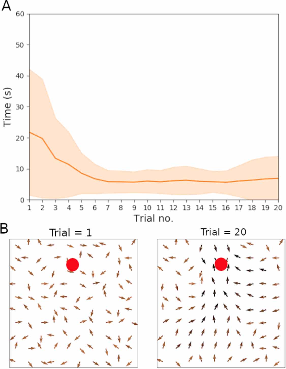
We first demonstrate the functionality of the learning rule (equations (18) and (19)), without reverse replays. Figure 2(A) shows the results for the time taken to reach the hidden goal as a function of trial number, averaged across 20 independent experiments. The time to reach the goal approaches the asymptotic performance after around five trials. Note, however, that there appears to be a larger variance towards the final two trials. Further trials were later run to test whether this increased variability in performance was significant or not (see section 3.2.4). Figure 2(B) displays the weight vector for the weights projecting from the place cells to the action cells. We note that after 20 trials, the arrows, in general, point towards the direction of the goal.

Figure 2. Results for the non-replay case to test that the derived learning rule performs well. Parameters used were η = 0.01 and  s. (A) Plot showing the average time to reach the goal (red line) and standard deviations (shaded area) over 20 trials. Averages and standard deviations are computed from 20 independent experiments. (B) Weight population vectors at the start of trial one versus at the end of trial 20 in an example experiment. Magnitudes for the vectors are represented as a shade of colour; the darker the shade, the larger the magnitude. Red dots indicate the goal location.
Download figure:
Standard image High-resolution image3.2. Effect of reverse replays on performance
We then ran the model with reverse replays, implementing the learning rule of equations (20) and (21), using first the same learning rate and eligibility trace time constant as in the non-replay case above. The performance average did not show differences by eye inspection. Further, a Wilcoxon Signed-Rank Test did not indicate any differences in the medians of the distributions with/without replay (p > 0.05 across 18 trials). The average time to reach the goal over the last ten trials is 6.21 s in the non-replay case and 6.92 s in the replay case (data not shown, see supplementary material). This result suggests in the first instance that replays are at least as good compared to the best-case non-replay, which was confirmed when comparing individually optimised parameters (learning rate and eligibility time constant) for each network.
In general, replays provide an additional source of information concerning the desirable synaptic changes. If the eligibility time constant is sufficiently large for the problem at hand but not too large to introduce instabilities, we would not necessarily expect to see any advantage. We expect to see an advantage when the eligibility time constant is too large for the problem or there is noise, for instance, high learning rates. Further results on the performance of varying the learning rate and eligibility trace time constant are presented next.
3.2.1. Reducing the eligibility trace time constant
The non-replay model requires the recent history to be stored in the eligibility trace. Having too short an eligibility trace time constant might negatively impact the model's performance. The time constant reflects how far back the information about the Reward will be 'transmitted'. Reverse replays, however, have the potential to compensate for this issue since the recent history is also stored and then replayed in the place cell network. Figure 3 shows the effects on performance of significantly reducing the eligibility trace time constant (to τ = 0.04 s). Both cases, with and without reverse replays, are compared. If the learning rate is too low (η = 0.01), then for neither case is there any learning. But as the learning rate increases, having reverse replays has significantly improved performance. Similar results are true for a larger, but not too large, eligibility trace time constant of  s (see supplementary material). Replays offer the most significant advantage when the eligibility trace time constant,
  , is relatively small. As this time constant gets larger, replays offer little to no performance advantage over non-replays (see supplementary material) when the maximum learning time is 20 trials (but see section 3.2.4 for a higher number of trials).

Figure 3. Comparing the effects of a small eligibility trace time constant with and without reverse replays.  s across all figures. Thick lines are averages across 40 independent experiments, with shaded areas representing one standard deviation. Moving averages, with a window length of three trials, are plotted here for smoothness.
Download figure:
Standard image High-resolution image3.2.2. Comparing differences in synaptic weight changes
There is an interesting comparison between the magnitudes of weight changes for the replay and non-replay cases. Figure 4 shows the population vectors of the weights after reward retrieval. Population vectors for the weights are computed according to equations (22) and (23). There are two observations to be made here. First, the weight magnitudes are greater with reverse replays, which is not surprising since activity replay results in more synaptic changes. And second is that the direction of the population weight vectors themselves is slightly different, particularly in the location at the start of the trajectory. In particular, the weight vectors point more towards the goal location in the replay case, whereas the non-replay case has weight vectors pointing along the direction of the path taken by the robot. Whilst we depict only one case here, this is representative of several cases for various parameter values.

Figure 4. Population weight vectors after reward retrieval in the non-replay and replay cases. The top figure shows the path taken by MiRo, where S represents the starting location and G is the goal location. Plots show weight population vectors for the non-replay case (A) and standard replay case (B) with  s; η = 0.1. The colour scale represents the magnitudes for each weight vector.
Download figure:
Standard image High-resolution image3.2.3. Performance across parameter space
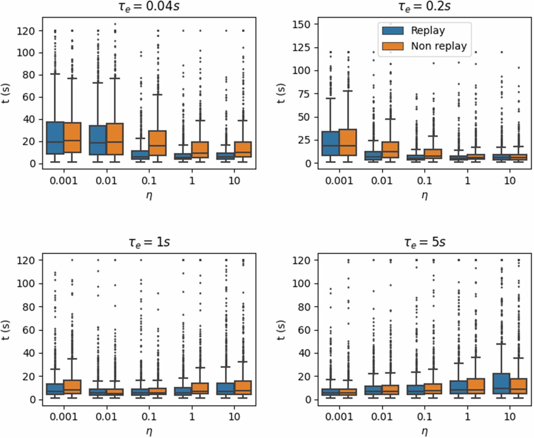
We investigated the robustness of the performance across various values of  and η. Figure 5 displays the average performance over trials 11–20, comparing again with replays versus without replays. There are perhaps two noticeable observations to make here. Firstly, when the eligibility trace time constant is small, employing reverse replays shows considerable improvements in performance over the non-replay case across the various values of learning rates. Learning still exists in the non-replay case; however, it is noticeably diminished compared with the replay case. Secondly, although this marked performance improvement vanishes for larger eligibility trace time constants, reverse replays do not hinder performance at the very least. To better interpret the results, it is essential to recall that learning rate and eligibility trace are multiplicative terms defining the weight updates; see equation (19). The eligibility trace should be long enough to enable propagation to the initial locations of the trajectory. High values in synaptic changes can also lead to instabilities, so small learning rates compensate for this. In general, the most successful combinations are large eligibility trace time constants and low learning rates or vice versa. However, for the reverse replay case, the additional information from the replay helps to perform well even in the case of a small eligibility trace time constant, as long as the learning rate is sufficiently large.

Figure 5. Comparing average performance across a range of values for  and η. Bars show the average time taken to reach the goal averaged across 40 independent experiments (as shown in figure 3 for instance) over the last ten trials (i.e. trials 11–20) shown as box plots. On each box, the central mark indicates the median, and the bottom and top edges of the box indicate quartiles Q1 and Q3. The whiskers extend 1.5 times the interquartile range (Q3–Q1); everything outside this range is an outlier.
Download figure:
Standard image High-resolution image3.2.4. Comparison of best cases
Figure 6 compares the results for the best cases with and without reverse replays. We optimised  and η independently for each case and ran 30 trials to achieve these results. The reason for this was a suspected instability in the non-replay case, i.e. a drop in performance as learning continues above the 20 trials. We interpret this as an advantage of the replay case in terms of stability rather than performance.

Figure 6. Comparing the best cases with and without reverse replays. With reverse replays the parameters are  s, η = 1. Without reverse replays the parameters are
  s, η = 0.01. The means (solid lines) and standard deviations (shaded regions) are computed across 40 independent experiments.
Download figure:
Standard image High-resolution image
In figure 2, where in trial 20 and above, the time to complete the task increases without replay but not in the case with replay. A Wilcoxon signed-rank test on the trials supported that data for the two conditions do not have the same median for 8 of the last 12 trials (p < 0.05, the complete table of results is in the
We also note the significant difference in the optimal parameters for the best cases with/without replay. With reverse replays the parameters are  s, η = 1, whereas without reverse replays they are
  s, η = 0.01. We speculate that the necessary choice in the eligibility time constant for the non-replay case (i.e. it needs to be large enough to store the trajectory history) underlines the cause of this instability. On the contrary, the reversal reply introduces additional synaptic changes, allowing for smaller eligibility time constants and helping the rule stability.
4. Discussion
Hippocampal reverse replay has long been implicated in RL [12], but how the dynamics of hippocampal replay produce behavioural changes and why hippocampal replay could be significant in learning are open questions. We have been able to examine the link between hippocampal replay and behavioural changes in a spatial navigation task by embodying a hippocampal-striatal inspired model [59] into a simulated MiRo robot and then augmenting it with a model of hippocampal reverse replay [64]. We have shown that reverse replays generate more robust behavioural trajectories over repeated trials.
In the three-factor synaptic eligibility trace hypothesis, the time constants for the traces have been argued to be on the order of a few seconds, necessary for learning over behavioural time scales [15]. However, results here indicate that due to reverse replays, synaptic eligibility trace time constants do not need to be on the order of seconds—a few milliseconds are sufficient for our task. The synaptic eligibility trace is still required here to store the history and inform the reverse replay mechanism; enough information is required for an effective reinstatement during a reverse replay. It has also been argued that neuronal, as opposed to synaptic, eligibility traces could be sufficient for storing a memory trace, as in the two-compartmental neuron model of [5]. Intrinsic plasticity in this model is not unlike a neuronal eligibility trace, storing the memory trace within the place cells for reinstatement at the end of a rewarding episode.
It could be the case that reverse replays stabilise learning by introducing an additional source of information regarding past states (an additional eligibility trace). The results shown here support this. Experimental evidence shows that disruption of hippocampal ripples during awake states, when reverse replays occur, disrupts but does not entirely diminish spatial learning in rats [27]. Whilst the longer eligibility trace time constants in this model ( in the range of 1–5 s) do not show diminished performance without reverse replays, the smaller time constants (
 in the range of 0.04–0.2 s) do. Hence, these results support the view that reverse replays enhance, rather than provide entirely, the mechanism for learning. Beyond reverse replays, however, forward replays have been known to occur on multiple occasions for up to 10 h post-exploration [17], which could be more important for memory consolidation than awake reverse replays [10, 16].
In the best case comparison (figure 6), we can understand why a sufficiently large, yet not overly large, eligibility trace time constant for the non-replay case gives the best performance. It must store a suitable amount of the trajectory history for learning. If the eligibility trace time constant were too small in relation to the length of the trajectory, it would not store enough of the history, whereas too large and it would store sub-optimal or unnecessary trajectories that go too far back in time. Yet the non-replay model became more unstable as the number of trials increased, as shown in figure 6. One explanation is that the eligibility trace time constant necessary for learning in non-replay had to be large enough to store trajectory histories. This necessity increases the probability that the robot learns sub-optimal paths. However, since the trajectory was replayed during learning, it was not necessary to have such a large eligibility trace time constant for the replay case. Therefore, suboptimal paths going back in time are quickly forgotten. Furthermore, replays can slightly modify behavioural trajectories. By looking at the effects in the weight vectors of figure 4, it is apparent that the weight vectors closer to the start location are shifted to point more towards the goal in the replay case.
Ultimately, our model makes several simplifications. Like [59], we assume the formation of the place cells before the task. Hence the robot has been previously familiarised with the environment. There are existing models able to demonstrate the formation of place cells from visual input; see, for instance, work from [55]. While the model assumes prior knowledge of the environment, the robot does not know the location or meaning of obstacles (walls). It learns these with the homing task via the administration of negative rewards, again similar to [59]. This approach is often taken in theoretical RL studies though it may not be accurate for a living creature. Arguably, a living creature would be aware of the significance of boundaries and would avoid moving into obstacles. Similarly, a robot may have a separate local navigation module that would generate a course diversion to avoid hitting objects. We have previously demonstrated how this local navigation could be acquired through RL [35, 48]. More generally, control architectures in both animals and robots are likely to distinguish between the global and local navigation problems and employ separate mechanisms for each [44].
We further assume that the reference system used in the study is allocentric. While it is a common belief that spacial signals within the hippocampus are allocentric, recent studies provide evidence of egocentric processing [62]. Parietal cortex neurons likely perform egocentric–allocentric coordinate transformation [6]. For a detailed model explaining place cell formation, see [34]. Our bio-inspired model adopts biological elements and explores their interplay in an artificial setup, a robotic simulation. As such, we have allowed ourselves to tuning parameters that may not be consistent with biological ones. Further, we mathematically derived our learning rule from objective functions, albeit we made sure to impose assumptions for simplicity, i.e. ensuring a uniform learning rule for both the learning and reference replay phase. Hence, the details may not closely resemble biology. However, we think it is an appropriate model for studying the potential advantages of reverse replay in RL. We envisage improving the biological plausibility by combining with models such as [34] and constraint parameters in appropriate regimes, though we feel this is beyond the scope of this work.
In our model, there are two sets of competing behaviours during the exploratory stage: the memory-guided behaviour of the hippocampus and the semi-random walk behaviour—heuristically selected based on the signal strength of the hippocampal output. If the hippocampal output does not express strongly for a particular action, we use the semi-random walk behaviour. An interesting comparison with the basal ganglia, and its input structure, the striatum, could be made here since these structures likely play a role in action selection [19, 37, 46, 50]. A fundamental interpretation of this action selection mechanism is that the basal ganglia receive a variety of candidate motor behaviours, which are perhaps mutually incompatible, but from which the basal ganglia must select one (or more) of these behaviours for expressing [20, 21]. Since the selection of action in our model is determined from the striatal action cell outputs, it appears likely that this selection would occur within the basal ganglia.
A further interesting observation is that, in the synaptic learning rule presented here, the difference between the action selected, yi
, and the mean of the distribution of the hippocampal output,  , is used to update synaptic strengths. Assuming that our mathematically derived rule is consistent with the biology, one interpretation could be that this difference behaves as an error signal, signalling to the hippocampal-striatal synapses how 'good' or how 'close' their predictions were in generating behaviours that led toward rewards. But how might this be implemented in the basal ganglia? While the striatum acts as the input structure to the basal ganglia, the neuroanatomical evidence shows that the basal ganglia sub-regions loop back on one another [20]. In particular, the striatum sends inhibitory signals to the substantia nigra, which in turn projects back both excitatory and inhibitory signals via dopamine (D1 and D2 receptors, respectively) to the striatum [14, 23]. There is a potential mechanism for appropriate feedback to the hippocampal-striatal synapses to provide this error signalling. Exploring this error signal hypothesis could be a potentially exciting research endeavour.
5. Conclusion
This work has explored reverse replays' role in biological RL. As a baseline, we have derived a policy-gradient RL rule, which we employed to associate actions with place cell activities and a corresponding supervised rule of the same form, where we interpret replay activities as frequency targets for the neurons. The result is a three-factor learning rule with an eligibility trace, where the eligibility trace stores the pairwise co-activities of place and action cells. We demonstrate the performance of the proposed learning rule in a simulated MiRo robot for a task inspired by the Morris water maze. We further augmented the network and learning rule with reverse replays, which acted to reinstate recent place and action cell activities. Because the reverse replays serve as a second source of information for the synaptic modifications (in addition to eligibility traces), they allow for smaller eligibility trace time scales and higher learning rates. Our results suggest that this additional source of information also helps with stability issues that our policy gradient rule demonstrates when we allow learning to take place for an increased number of trials. Our results postulate that reverse replay may enhance RL in the hippocampal-striatal network whilst not necessarily providing its sole mechanism.
Acknowledgments
The authors thank Andy Philippides and Michael Mangan for their valuable input and useful discussions.
Data availability statement
The data that support the findings of this study are openly available at the following URL: https://github.com/aljiro/robotic_RL_replay.
Conflict of interest
TJP is a director and shareholder of Consequential Robotics ltd, the company that developed and markets the MiRo (MiRo-e) robot; he is also a director/shareholder of Cyberselves universal ltd, which develops robotic middleware. All other authors declare that the research was conducted in the absence of any commercial or financial relationships that could be construed as a potential conflict of interest.
Author contributions
M T W, T J P, and E V conceived and planned the study. M T W conceptualised the interactions of activity replay and reinforcement learning, developed the computational model and conducted the initial simulations. E V derived the reinforcement and supervised learning rules and co-designed with M T W the simulation experiments. A J R performed additional simulations. M T W and E V drafted the initial manuscript. All authors contributed to the manuscript revision.
Funding
This work has partly been funded by the EU Horizon 2020 programme through the FET Flagship Human Brain Project (HBP-SGA2: 785907; HBP-SGA3: 945539) and by EPSRC EP/S030964/1.
Appendix
Appendix. Mathematical derivation of the place-action cell synaptic learning rule
Derivation of the reinforcement learning rule
We derive a policy gradient rule [57] following [59], but here we use continuous valued neurons instead of spiking neurons. The expectation for the rewards earned in an episode of duration T is given by,

where X is the space of the inputs of and Y the space of the output of the network, and  the probability that the network has input x and output y, parametrised by the weights.
We can decompose the probability,  (see decomposition of the probability in [59]) as,

where hi
is the probability the ith action cell generates output  contained in y, when the network receives input x. Similarly gj
is the probability for the activity produced by the jth place cell given its input. We then wish to calculate the partial derivative over a weight wkl
of the expected reward,
contained in y, when the network receives input x. Similarly gj
is the probability for the activity produced by the jth place cell given its input. We then wish to calculate the partial derivative over a weight wkl
of the expected reward,

To do so, we take into account that ![$P_w\left({\mathbf{x}},{\mathbf{y}}\right) = \left[ \frac{P_w\left({\mathbf{x}},{\mathbf{y}}\right)}{h_k\left({\mathbf{x}},{\mathbf{y}} \right)} \right]h_k\left({\mathbf{x}},{\mathbf{y}}\right)$](https://content.cld.iop.org/journals/1748-3190/18/1/015007/revision3/bbac9ffcieqn85.gif) , where the term in square brackets does not depend on wkl
since we remove its contribution from
, where the term in square brackets does not depend on wkl
since we remove its contribution from  by dividing with
  . We can then write,

This leads to,

To proceed, we need to consider the distribution of the activities of the action cells hk
. This we choose to be a Gaussian function with mean  and variance σ2 (see also section 'Striatal Action Cells'),

The mean of the distribution is calculated by  , see also equation (11), where fs
is a sigmoidal function. We note that a different choice of function would have resulted in a variant of this rule. Therefore,
, see also equation (11), where fs
is a sigmoidal function. We note that a different choice of function would have resulted in a variant of this rule. Therefore,

Replacing (31) in (29) we end up with,

Then the batch update rule is given by:

with the factor c1 absorbed in the learning rate.
The batch rule indicates that we need to average the term  across many trials. When an on-line setting is considered, the average is naturally rising from sampling throughout the episodes. Hence the on-line version of this rule is given by:

We note however that this rule is appropriate for scenarios where reward is immediate. To deal with cases of distant rewards, such as ours where reward comes at the end of a sequence of actions, we need to resort to eligibility traces. Our rule is similar to REINFORCE with multiparameter distribution [65]; we differ by having a continuous time formulation and a different parametrisation of the neuronal probability density function. Further, in our case we do not learn the variance of the probability density function.
We introduce an eligibility trace by updating the weights connecting the place cells to the action cells,  by:
by:

The term eij represents the eligibility trace, see also [57], and is a time decaying function of the potential weight changes, determined by:

Derivation of the supervised learning rule
During replays, we assume that synapses between place and action cells change to minimise the function:

in other words, we assume that during the replay equation (17) provides a fixed target value for the mean of the Gaussian distribution of the action cells at time t. In what follows we consider the target constant for the sake of the derivation and consistency with the form of the RL rule, but in fact this target changes as time and consequently the weights from place to action cells change, making the rule unstable, but stabilising under a short, fixed length of reply time. Taking the gradient over the error function with respect to the weight wkl , when considering the 'target' activity for the action cells fixed, leads to the backpropagation update rule for a single layer network:

where  is the learning rule, in our simulations
  similar to the RL rule. Also for consistency with the RL rule formulation, we introduce an eligibility trace by updating the weights connecting the place cells to the action cells,
  by:
by:

where the eligibility trace is determined by:

where again the time constant τe is the same as in the RL rule.
In the case of replays then, when the robot has reached its target, it first learns using the standard learning rule as in equations (35) and (36). After 1 s, a replay event is initiated, and learning is then done using the supervised learning rule here, using equations (39) and (40). By setting the reward value to R = 1, we can ensure that both the RL learning rule and the supervised learning rule become identical. Alternatively, a different value of the reward would require setting  .
.
Appendix. Best case comparison table of results
The table of results for the best case comparison shown in figure 6 is given here. The p-value for each trial is given. Cases where p < 0.05, are highlighted in bold.
| Trial no. | p-Value |
|---|---|
| 15 | 0.121 |
| 16 | 0.40 129 |
| 17 | 0.32 997 |
| 18 | 0.2177 |
| 19 | 0.0099 |
| 20 | 0.47 608 |
| 21 | 0.03074 |
| 22 | 0.0057 |
| 23 | 0.00776 |
| 24 | 0.04272 |
| 25 | 0.01539 |
| 26 | 0.15625 |
| 27 | 0.0057 |
| 28 | 0.015 |
| 29 | 0.18141 |
| 30 | 0.05592 |
Supplementary data (0.8 MB PDF)