

Abstract
Flight initiation is fundamental for survival, escape from predators and lifting payload from one place to another in biological fliers and can be broadly classified into jumping and non-jumping takeoffs. During jumping takeoffs, the legs generate most of the initial impulse. Whereas the wings generate most of the forces in non-jumping takeoffs, which are usually voluntary, slow, and stable. It is of great interest to understand how these non-jumping takeoffs occur and what strategies insects use to generate large amount of forces required for this highly demanding flight initiation mode. Here, for the first time, we report accurate wing and body kinematics measurements of a damselfly during a non-jumping takeoff. Furthermore, using a high fidelity computational fluid dynamics simulation, we identify the 3D flow features and compute the wing aerodynamics forces to unravel the key mechanisms responsible for generating large flight forces. Our numerical results show that a damselfly generates about three times its body weight during the first half-stroke for liftoff. In generating these forces, the wings flap through a steeply inclined stroke plane with respect to the horizon, slicing through the air at high angles of attack (45°–50°). Consequently, a leading edge vortex (LEV) is formed during both the downstroke and upstroke on all the four wings. The formation of the LEV, however, is inhibited in the subsequent upstrokes following takeoff. Accordingly, we observe a drastic reduction in the magnitude of the aerodynamic force, signifying the importance of LEV in augmenting force production. Our analysis also shows that forewing-hindwing interaction plays a favorable role in enhancing both lift and thrust production during takeoff.
Export citation and abstract BibTeX RIS
1. Introduction
Most forms of flight are initiated by a takeoff. From airplanes to birds, bats and insects, all share this common behavior. Particularly, for living organisms, takeoff is essential for survival, escape from predators and lifting payload from one flower to another during pollination, etc. For scientists and engineers, emphasis is placed on understanding the behavioral mechanisms during flight initiation in order to apply the findings to applications such as micro-aerial vehicle (MAV) design [1].
In understanding flight initiation, a lot of research has focused on jumping takeoffs of locusts [2], crickets [3], fruit flies [4], leafhopper insects [5] and birds [6, 7] where the forces generated by the legs are harnessed to accelerate the body away from the ground for flight initiation. Pond [2], showed that during jumping takeoff of the locust (Schistocerca gregaria), the body is clear of the takeoff platform by several body lengths before wing motion occurs. The mean latency (delay between when body took off from the platform and when wings began to move) in still air was reported to occur at about 33.2 ± 12.8 ms indicating that the wings do not actively contribute to the takeoff. However, a few studies have analyzed non-jumping takeoffs of insects. During non-jumping takeoffs, majority of the flight forces are generated by the wings and the body motion is slow in comparison to those achieved during jumping takeoffs. These slow takeoffs are more stable since the rotational velocities of the body are not too high to induce tumbling in the insect [4, 8].
Truong et al [9], analyzed a non-jumping takeoff of a rhinoceros beetle (flapping frequency ~ 37–38 Hz). The authors observed that takeoff occurred at the end of the third wing beat (WB). The impulse produced during the first wing beat was not sufficient to ensure liftoff. By modulating the pitch angle/geometric angle of attack of the wing and increasing flapping frequency, the insect achieved liftoff with the hindwings generating most of the necessary forces for flight. Additionally, Chen et al [8], studied a smooth slow takeoff of drone flies. For this high flapping frequency insect (~170 Hz), the legs left the ground after the thirteenth wing beat. Prior to liftoff, the aerodynamic forces increased to a value greater than the body weight while the flapping amplitudes also increased gradually and the leg forces decreased monotonically. In both papers [8, 9], the insects pitched up while ascending during flight initiation. However, these studies although essential, did not identify the important flow features and their link to wing kinematics and aerodynamic mechanisms that enabled flight initiation.
Here, we study the takeoff of a damselfly (flapping frequency ~27–28 Hz). Damselflies are known to initiate flight solely by flapping their wings [10]. However, none but one study has focused on an aspect of the takeoff mechanism of damselflies. Marden [10], measured the maximum payload a damselfly can carry during takeoff to determine the maximum lift production of the wings in still air. The maximum lift per unit mass ranged between 21.5–50 N kg−1. Nevertheless, no information on the wing kinematics or further aerodynamic data was provided. Conversely, the wing kinematics of damselflies have been previously reported in a few other studies which focus on forward [11, 12] and maneuvering flight [13, 14]. These studies showed that damselflies are capable of fine-tuning their wing kinematics to achieve extraordinary flight capabilities. For instance, free flight measurements on three different species of damselfly have shown that damselflies can perform yaw turns, ranging between 120–180°, within a few wingbeats [13, 14]. While our measurements on the wing and body kinematics of damselfly are in line with those previous findings, they reveal new flight capabilities of this insect such as voluntary flight initiation and liftoff within only one wingbeat.
Here, we aim to investigate the connection between the wing kinematics adjustments and aerodynamic force generation in the highly demanding flight condition of takeoff. To reconcile the relationship between the flapping motion of wings and the corresponding force production, some unsteady aerodynamic mechanisms have been previously suggested such as absence of stall/delayed stall, clap and fling, rotational circulation and wing-wake interactions [15]. Among these, the leading edge vortex (LEV) is the most potent and has been observed in multiple insect species such as hawkmoths [16, 17], bumblebees [18], and dragonflies [19]. The LEV is responsible for about two-thirds of the total lift force in insect flight [20] but has just recently been measured in free flying hawkmoths in forward flight [16]. Most previous studies have been based on tethered flight and had not focused on the role of the LEV during flight initiation. The LEV enhances lift by adding its circulation to the bound circulation of the wing [21]. The LEV is usually stably attached to the wing's surface and breaks down towards the end of the stroke. So far, the presence of LEVs has been extensively reported in the downstroke phase of flight. Conversely, a small LEV (or the absence thereof) or attached flow has been reported during the upstroke phase of flight as well as on the hindwings of dragonflies [17, 19, 22, 23].
Apart from the LEV, another important unsteady mechanism relevant to takeoff is 'clap and fling'. Fling was observed as a mechanism for generating large forces in butterfly takeoff [24]. Fling eliminates slow development of circulation but creates large circulation values independent of wing translation or the Wagner effect [15, 25]. When weights were attached to damselflies during takeoff, they used the mechanism [10]. However, in free flight with no attached payload, the mechanism was not used [12, 26]. Other insects also choose to shun this mechanism [26].
Our work adds to a handful of studies on damselflies (Zygoptera) flight mechanics [10, 12, 13]. Previously used quantifications of force and unsteady effects involve the local circulation method (LCM) for circulation measurement and quasi-steady models for approximating the force [12, 13, 27]. PIV has also been used to study model wings, tethered flight of insects, the free flight of birds and bats and recently free flight of Hawkmoth and dragonflies [6, 16, 20, 23, 28–32]. For the first time, however, using a high fidelity CFD simulation, we are able to identify the 3D flow features of a damselfly during takeoff. Furthermore, we discuss unique wing and body kinematics not previously mentioned in damselfly literature. And finally, we elucidate how the kinematics influences the aerodynamics to ensure a successful flight.
2. Materials and methods
2.1. Damselflies, high speed photogrammetry and 3D surface reconstruction
Damselflies (Hetaerina Americana) were caught outside during the summer of 2012 in Dayton, Ohio for experiments. Prior to the experiments, the caught damselflies' wings were dotted for tracking purposes (figure 1). The video footages were then recorded shortly after their capture in a quiescent environment of about room temperature (70 °F) in order to prevent inactivity during the time of experiments.
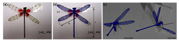
Figure 1. Damselfly species with morphological parameters. (a) A representative of the damselfly (Hetaerina Americana) in this study is shown. (b) An image of the reconstructed damselfly is overlapped on the real damselfly image. The dots are the marker points are placed on the wing for tracking the wing motion. Morphological parameters are also labelled.  is the mid-chord length, L is the damselfly body length, R is the wing length and d is the distance between the wing roots (0.465
 ). (c) Reconstruction technique in action on a high speed video of a damselfly in flight (unpublished). The side and top views are shown to indicate that details of wing deformation are captured during reconstruction.
Download figure:
Standard image High-resolution imageTable 1. Morphological data for the damselfly species in this experiment. The mass and length uncertainties are about ±1 mg and ±1 mm, respectively.
| Species | Body weight (mg) | Body length (mm) | Forewing length (mm) | Forewing chord (mm) | Hindwing length (mm) | Hindwing chord (mm) | Wing area (mm2) | Flapping frequency (Hz) |
|---|---|---|---|---|---|---|---|---|
| Hetaerina Americana | 75 | 42 | 29 | 6 | 29 | 6 | 136 | 27 |
The damselflies initiated flight autonomously in the shooting area. Their flight triggered a photogrammetry setup consisting of three orthogonally arranged and synchronized cameras shooting at 1000 frames per second (fps). After recording the flight, the wings were removed and morphological parameters were measured (see table 1). We selected one of the recorded footages for analysis. In this recording, the damselfly initiated flight from a pitch down body orientation and flew upward and forward thereafter. The dotted wings of the insect were tracked manually frame by frame in Autodesk Maya (Autodesk Inc.). Figure 1(b) shows a visual representation of the reconstructed insect placed on top of an image. Our surface reconstruction technique (shown in figure 1(c)) allows us to record and measure small deformations in the wing during flight (see section 2.2). We are capable of measuring wing twist and camber during flight. The accuracy of this reconstruction technique is discussed extensively in Koehler et al's work [33] and has been applied in the study of damselflies, dragonflies and cicadas [13, 34–37].
2.2. Wing kinematics and deformation metrics
The wing kinematics and deformations were measured by defining a least-square reference plane (LSRP) generated based on the points on the reconstructed wing surface. The LSRP is the plane of least wing deformation. For details of how the LSRP was calculated, see the work of Koehler et al [33]. A mean stroke plane was also defined based on the average trajectory wing tip per stroke. The orientation of the wing in the stroke plane is described by three Euler angles; flap, deviation and pitch. Flapping motion is the revolution of the wing in a back and forth manner and is positive during the downstroke. The up and down rotations with respect to the stroke plane is expressed by the deviation angle as is positive when the wing is above the stroke plane. The wing pitch angle is characterized by the rotation of the wing about its pitching axis close to the leading edge. The pitch angle is measured clockwise from the intersection between the LSRP and the line defining the stroke plane hence varies between 0° and 180°. The geometric angle of attack (AoAgeom or  ), is defined as the angle between the normal to LSRP and the normal to the stroke plane and is equivalent to the wing pitch. The effective angle of attack (AoAeff or
  ), is the angle between the wing and the incident flow upon it. For wing deformation metrics, the local twist angle is reported. The twist angle is the relative angle of the deformed wing chord line with a rigid plane of reference defined as the LSRP. Since the surface of the wing is deformed and twisted, the local angle of the chord line with LSRP varies along the wing span. Thus, we use the term 'local twist angle' to emphasize that the orientation of the wing surface relative to the rigid plane of reference is not constant and varies along the span. Visual representations of these definitions are rendered in figure 2.

Figure 2. Definition of the kinematics parameters. (a) Wing kinematics. The Euler angles of the wings in the stroke plane; flap, pitch and deviation are denoted by  ,
,  , and
, and  respectively. The green arrows represent a coordinate system placed at the wing root.
  is the effective angle of attack. The angle between the normal to the chord (cyan arrow) and the normal to the stroke plane (purple arrow) is equivalent to the pitch angle or the geometric angle of attack (AoAgeom). (b) Body kinematics. The coordinate system is fixed at the center of mass. Roll, pitch and yaw are denoted by
  ,
,  and
and  respectively. (c) Twist angle measurement. The deformed wing is shown in blue whereas the LSRP i.e. the plane of least deformation, has the least deformed wing project on it in light gray with a red outline. Two dimensional (2D) cross-sections are taken along the wing length and the angle between the chord line of the least deformed wing (dashed line) and deformed wing (solid line with red tip) is the twist angle of the wing. Two of those 2D slices are shown to indicate the variation of twist along the wing length.
Download figure:
Standard image High-resolution image2.3. CFD simulation
To elucidate the flow field around the damselfly in flight, we obtained the flow information from computational simulations. A high fidelity CFD solver based on the immersed boundary method was used in this study. We solved the incompressible viscous Navier–Stokes equation (equation (1)) using a finite difference method with 2nd order accuracy in space and a 2nd order fractional step methods for progressing in time. More details of this method and its application in studies on dragonflies and cicadas can be found in [33, 35, 38].
Here u is the velocity vector,  is the density,
  is the kinematic viscosity and
  is the pressure.
The vortex structures were characterized by the Q-criterion [39] shown below.
Here ![$\mathbf{S} ~\text{=} ~ \frac{1}{2}\left[\nabla \mathbf{u}+{{\left(\nabla \mathbf{u}\right)}^{\text{T}}}\right]$](https://content.cld.iop.org/journals/1748-3190/12/5/056006/revision2/bbaa7f52ieqn015.gif) and
and ![$\boldsymbol{\Omega } ~\text{=} ~ \frac{1}{2}\left[\nabla \mathbf{u}-{{\left(\nabla \mathbf{u}\right)}^{\text{T}}}\right]$](https://content.cld.iop.org/journals/1748-3190/12/5/056006/revision2/bbaa7f52ieqn016.gif) are the strain rate and vorticity tensors respectively. More details on the flow visualization techniques are shown in Koehler et a's work [40].
are the strain rate and vorticity tensors respectively. More details on the flow visualization techniques are shown in Koehler et a's work [40].
The simulation was run on a non-uniform Cartesian grid. The computational domain size was about 50 × 50
× 50 × 50
× 50  with about 13.8 million grid points in total. The high resolution uniform grids surround the insect in a volume of 14.5
 × 12
× 12 × 13.5
 with a spacing of about 0.06
 . This ensured sufficient resolution for capturing the 3D flow field. The stretching grids move in all three directions from the fine region to the outermost boundaries. The boundary conditions of the domain on all sides are zero gradient.
The Reynolds number for the flight is defined by  and is 1220. It is measured based on the average wing tip speed (
 ), mid-chord length (
 ), kinematic viscosity of air at room temperature (
 ). Validation for the flow solver can be found in recent works by Wan et al [38] and Li and Dong [36].
The current grid set-up was selected based on checks to ensure the grids are refined to preclude grid dependence of the simulation. Figure 3(b) shows the comparison of the lift coefficient history of the second flapping stroke in three grids (coarse, medium and fine). The difference of both the mean value and the peak value of lift between the medium-grid case (adopted in this paper) and the fine-grid case is about 2%, thereby, establishing that the aerodynamic force calculations in the current study were grid-independent.

Figure 3. CFD simulation setup. (a) This figure shows the schematic of the computational mesh and boundary conditions employed in the current simulation for the damselfly flight. For ease of the display, the meshes are made less dense four times in each direction. (b) Grid independent study. The coefficient of lift is shown during the second flapping stroke. The gray shading indicates the downstroke of the forewings. Coarse = 9.8 million; medium = 13.8 million; fine = 15 million. The medium grids are shown in (a).
Download figure:
Standard image High-resolution image3. Results
3.1. Kinematics
3.1.1. Body kinematics
To evaluate flight behavior during and after flight initiation, we studied the kinematics based on the reconstruction output. Figure 4(a), shows the body motion of the damselfly during the takeoff stage of flight. After being stationary for some time, the wings begin to slowly peel off during the preparatory stages before initiating takeoff. The preparatory stage lasted for 30 ms. During the preparatory stage, the insect adjusted both the stroke plane of the wings relative to the body and the pitch angle of the body. At the start of the takeoff, the body was at a pitch down orientation (about −50°). Liftoff, defined as the time duration within which the legs of the insect leave the platform, starts with the wings moving downward in a steep stroke plane. The whole takeoff encompasses the up and downstroke of the wing during the first flapping stroke. Our observation suggests that legs do not play a significant role in pushing the body up. It takes less than a wingbeat for the insect to get airborne. This is a relatively short time among the insects which do not jump to initiate flight [8]. The peak vertical acceleration measured based on the center of mass motion during liftoff was about 3 g. The value was less than the vertical acceleration for fruit fly takeoff (6 g) [4] and butterfly takeoff (10 g) [24].
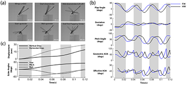
Figure 4. Kinematic events during an autonomous takeoff in a damselfly (Hetaerina Americana; body weight = 0.735·mN). (a) A series of images depicting the sequence of events during the takeoff stroke. (b) Wing kinematics. The kinematics are reported in the stroke plane. The definitions of the angles are in figure 2. The angles of attack are reported at mid-span (c). Body kinematics. The top figure shows the displament of the insect during flight. The bottom figure shows the body Euler angles.
Download figure:
Standard image High-resolution imageThe total takeoff duration is about 45 ms and the direction of motion is up and forward while the damselfly also turns slightly. Nevertheless, the translational displacement is significantly higher than the rotational displacement. The focus of our work is on the translational displacement. The mean body Euler angles during the first wing beat are −5.5°, 46.6°, 8.4° and the maximum rotational velocities during the first wing beat 500° s−1 and 200° s−1 for roll, pitch and yaw respectively. The takeoff is slow and stable and no tumbling was observed [8]. The body was kept straight and no body deformations were obvious. We include two subsequent flapping strokes in our analysis to document latter events during flight. During the latter strokes, the damselfly ascends, travels further and attains a more horizontal posture as flight speed increases (figure 4(c)).
3.1.2. Wing kinematics and deformations
The average kinematics of the left and right wing measured in the stroke plane are shown in figure 4(b). The gray shading denotes the downstroke of the forewings. From the onset of flight, the motion of the fore and hind pairs of wings are offset by a slight phase difference that increases over time. The forewings (FW) lead the hind wings (HW) by about 26° in the initial stroke (takeoff stroke) and about 37° in the latter strokes (2nd and 3rd strokes) as shown in figure 4(b).
Averaged across the three flapping strokes, the wings sweep through a stroke plane that maintains an orientation of about 18.6 ± 5.3° for the forewings and 21.6 ± 6.1° for the hindwings, measured clockwise with respect to the longitudinal axis of the body. We will refer to this as the geometric stroke plane angle ( ).
).  is measured based on the trajectory of the wing tips. Wing kinematics including the geometric stroke plane vary from one stroke to the next, which indicates constant adjustment of the wing kinematics by the insect [11]. In the global orientation, due to steep body angle, the stroke plane with respect to the horizon (
 ) is heavily influenced. The fore and hind wings flap at a stroke plane angle of 49.8 ± 21.1° and 52.8 ± 21.4°, relative to the horizon, respectively, with the highest stroke plane inclination occurring in the takeoff stroke. At this instant, the stroke plane is titled steeply downwards while a less tilted stroke plane is utilized as the body becomes more horizontal in subsequent strokes. During the takeoff,
  are very similar both in up and downstroke with variations of a couple of degrees (1° for FW and 7° for HW), whereas the difference in other strokes is more obvious wherein downstroke stroke planes are more inclined than the upstroke (15° for FW and HW) due to a faster rate of change of body posture compared to
  .
.
In the first wing beat, the wings flap with the highest stroke amplitude recorded throughout the flight (120° and 140° for FW and HW respectively). At all times, the hindwings flap with a higher stroke amplitude (figure 4(b)). As the wings flap, they are oriented at high pitch angles/AoAgeom. The instantaneous values are shown in figure 4(b). The half-stroke average AoAgeom during the first downstroke is 51° and 65° for the fore and hindwings respectively. Whereas, the half-stroke average AoAgeom is 71° and 81° during the upstroke fore and hindwings respectively. During takeoff, it is evident that the hindwings flap at higher pitch both in the upstroke and downstroke. Though, in subsequent strokes, the forewings flap with higher pitch during the downstrokes (figure 4(b)). In latter upstrokes, the average pitch of the fore and hindwings are similar even though the hindwings still flap with greater stroke amplitude. The upstroke AoAgeom in the takeoff stroke is about 20° higher than the downstroke. Comparing the initial upstroke with latter upstrokes, the average upstroke AoAgeom is about 30–35° greater. On the contrary, the stroke average downstroke AoAgeom only varies by at most 13°. At reversal, the wings rotate and experience the highest AoA. During this period, the wings may generate instantaneous AoAgeom in excess of 90°.
The wings of damselflies are flexible, deforming and twisting as they flap through the air. The effective angle of attack ( ) measured at 0.5R is reported here, although
  is not sigificantly different at 0.7R and 0.9R (see figure 5(b)). The half-stroke average
  during the 1st downstroke is 44° and 45° for the fore and hindwings respectively. In the upstroke, half-stroke average
  and 45° and 51° for the fore and hindwings respectively. During the downstroke, the
  for the pair of wings is very similar, whereas in the upstroke, slight differences are evident with the hindwings having a slightly higher
  . Comparing the initial upstroke with latter upstrokes, the average upstroke
  is about 15° and 23° greater for the fore and hindwings respectively. On the contrary, the downstroke
  only varies by at most 6° and 11° for the fore and hindwings respectively. The effective angles of attack during this flight are higher than previously reported values. Sato et al [12] recorded a maximum
  of 15° for majority of the downstroke during forward flight of damselflies.
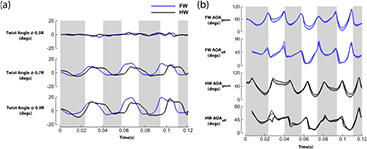
Figure 5. Local twist and AOA from mid-span to tip. (a) The local twist angle and (b) AoA at different spanwise locations (.50R,.70R,.90R) are reported here. Dashed lines = .50R, long dashed lines = .70R, dashed dot dot lines = .90R.
Download figure:
Standard image High-resolution imageFigure 5(a) shows the local twist along the wing. Three cross sections are chosen for display; 0.5R, 0.7R, 0.9R. Similar to the wing kinematics, the twist profiles of the wings are averaged between the left and right wings. The measured twist angle across the cross-sections is at most 20° and occurs at the cross-sections nearest to the wing tip (0.9R). The maximum twist recorded occurred during the mid-stroke with the forewings deforming more than the hindwings. The upstroke twist are also more significant than the downstroke's. The mid-chord of the wing (0.5R) has minimal twist.
3.2. Identification of vortical structures during takeoff flight
3.2.1. 3D flow structures
Having quantified the wing motions and deformations, here, we present the three-dimensional (3D) flow phenomena based on the CFD simulation to study how the wing motions and corresponding deformations influence the aerodynamic mechanisms responsible for force generation. Figure 6 shows the evolution of the wake structures in the takeoff stroke. The start, mid and end of the downstrokes and upstrokes are shown on the left and right columns respectively. The snapshots are selected based on the timing of the hindwings. This way, we can capture the details of both pairs of wings since the forewings lead by a small phase difference. The left wings are shown, however, the same flow phenomena occur on the right wings. The vortex structures are visualized by plotting the iso-surface of the Q-criterion. Two iso-surface values (Q = 3% and 6% of maximum Q) are chosen to identify the wake structures. The flow structures evident on both pairs of wings are mainly characterized by tip vortices (TV) and an LEV.
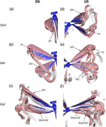
Figure 6. A time course of vortex development in the takeoff stroke. The vortical structures are visualized by the Q-criterion. The downstroke and upstroke are abbreviated as DS and US respectively. TEV = trailing edge vortex.
Download figure:
Standard image High-resolution imageAt the onset of the downstroke, a starting vortex sheet (SV) sheds from the trailing edge of the wing surface. Simultaneously, an LEV is formed due to wing translation both on the fore and hindwings. The vortex rapidly grows in size and strength as the wing flaps at high AoAs. The LEV remains attached to the wing surface till wing reversal when it is shed and another LEV develops for the first upstroke only, on the anatomical lower surface of the wing which has become the aerodynamic upper surface (figure 6(d)). We do not observe multiple LEVs rather a single LEV across the wing surface. The excess vorticity is concentrated near the tip and sheds into a strong trailing vortex. During the upstroke, an LEV develops immediately after completion of the downstroke in the first stroke only (figures 6(c) and (d)). The LEV actually forms first at the distal part of the wing where the combination of high wing pitch and velocity, consequently leads to high  , and causes flow separation. At about mid-stroke, an LEV covering the wing surface is observed (figure 6(e)). The LEV is similar in size to the first downstroke's LEV (figure 6(b)) at this instant. Therefore, the magnitude of circulation and thus the lift production capacity of the wing surface should be similar. The LEV remains attached to the surface and sheds during rotation.
3.2.1.1. A comparison of first and subsequent strokes
To understand the flow structures observed in the takeoff stroke, we compared the findings to the second flapping stroke. Figure 7 shows selected snapshots of the evolution of the near wake in the first two wing beats. These snapshots are taken at both the fore (top row) and hindwing (bottom row) mid-strokes.

Figure 7. Flow features at mid-stroke visualized by the Q-criterion. (a) and (b) Represent the flow features during the 1st stroke at the fore and hindwing mid-strokes respectively. (c) and (d) Represent the flow features during the 2nd stroke at the fore and hindwing mid-strokes respectively. Dashed circle in figure (d) shows the LEV formed as the wing approaches reversal.
Download figure:
Standard image High-resolution imageThe vortex structures on the wing during the downstrokes are similar. A well attached LEV is present on the wing surface and excess vorticity feeds into a TV. The upstroke is quite different, however. In comparison to the first stroke, an LEV is not observed during the translation of the wing in the second upstroke which indicates that the wing does not dynamically stall (figures 7(c) and (d)). However, an LEV appears for a short duration during the wing pronation due to rotation effects where the angle of attack increases rapidly as the wing rotates (figure 7(d)). The appearance of the LEV is for a short duration and cannot compensate for the inability of the wing to generate substantial lift during the translational part of the stroke. Due to the absence of an LEV, no excess vorticity spirals toward the tip. The wing simply translates with attached flows on its surface which is not visible with the Q-criterion. The vortical structures around the hindwings in (figure 7(d)), are the remnants of the shed LEV during the downstroke reversal of the second stroke originating from the anatomical dorsal surface of the wing.
3.3. LEV circulation
Having identified the vortex structures, the time history of the LEV circulation of the left wings presented in figure 8(c), is calculated at the mid-span of the wings shown in figure 7. The circulation is calculated by measuring the flux of the vorticity. To do so, at every time step of the numerical simulation, a 2D plane normal to the axis of LEV is constructed. A vorticity threshold is set (typical of Eulerian vortex identification methods) to capture the vortex boundaries. The circulation is calculated using equation (3).
where  is the vorticity. The area of integration (dS) is bound by the vorticity threshold and the circulation is non-dimensionalized by
  and
and  (figures 8(a)–(c)). The circulation curves lag behind the wing kinematics a bit due to the delay in vortex formation at the onset of flapping. A discontinuity in the curve exists around wing reversal because of the deterioration of one vortex and the emergence of another on opposite surfaces on the wing. The circulation grows from inception of flapping, attains a maximum around the mid-stroke region and begins to attenuate as reversal approaches. This is an indication of the evolution and strength of the vortex over time. Negative LEV circulation indicates clockwise rotation of vorticity and occurs during the downstroke. The reverse happens in upstroke.

Figure 8. Quantitative measurement of velocity and pressure difference on the wing surface. (a) Calculation of LEV circulation. A schematic of a damselfly with 2D slices on the wings with virtual cameras looking through a line passing through the LEV core. A magnified image of one of the slices is shown. The green boundary around the LEV shows the area in which the flux of vorticity is calculated. The boundary is determined by a vorticity threshold which defines the LEV. (b) Spanwise vorticity on FW. This is taken at mid-span of the takeoff stroke in the downstroke and upstroke respectively on the forewings. 2D slices are cut from the wing root to the wing tips and the vorticity is normalized by  . The circulation in (c) is calculated by taking the flux of the vorticity. (c) LEV circulation at mid-Span of the left wings. (d) Pressure difference on the wing surface. (e) Isosurface of pressure coefficient (
 ).
).
Download figure:
Standard image High-resolution imageThe total circulation as well as the fore and hind wing circulation in the 1st downstroke and upstroke are similar with the only difference being the rotational direction of the LEV. In subsequent strokes, another pattern emerges. The DS circulation is much higher than the US circulation. The hindwings, in general, have a higher circulation than the forewings over the course of the flight.
Since our method of calculating vorticity cannot distinguish between a vortex and the underlying shear layer, both on the wing surface and in between the vortices, we can attribute the circulation observed in the 2nd and 3rd US to the shear layer/attached flow or a very tiny and weak LEV in the subsequent upstrokes (see figures 7(c) and (d)).
3.4. Pressure distribution and correlation to flow structures
To probe further into how the flow structures affect the force distribution on the wing surface, the distribution of the pressure difference between the top and bottom surface of the left wings is shown in figure 8(d). We show the pressure distributions at exactly the same snapshot as figure 7. The pressure difference is projected onto a top view image of the wings for clarity. Moreover, the forewing mid-strokes are superimposed on the hindwing mid-strokes. The same range of contours is plotted for the 1st and 2nd stroke only for ease of comparison. The pressure is non-dimensionalized as  . The pressure difference distribution indicates what part of the wing produces the greatest velocity difference or circulation. The greatest pressure difference is generated on the distal part of the wing toward the wing tip in both US and DS. At this point, the tip speed is greatest.
When we compare the mid-upstrokes of both the 1st and 2nd strokes, we find drastic differences in the pressure distribution. Figure 8(d), shows the pressure difference contours with the darker shade (dark blue) contours indicating regions of low pressure difference. An observation of figure 8(d) indicates lower pressure difference distribution on the wing during the 2nd upstroke as compared to the 1st. Comparing the flap velocities of the wing in these two phases of flight (see figure 4(b)), we find their velocities to be similar with the 2nd upstroke's slightly higher. The major difference is in the pitch angle and  . In the second stroke, the instantaneous
  is as low as 7° and 11° for the fore and hindwings during translation, which means the flow, did not stall. Conversely, the instantaneous
  is as low as 29° and 46° for the fore and hindwings in the first upstroke, indicating flow separation at the leading edge of the wing. Figure 7, shows the presence of an LEV in the 1st upstroke and its absence in the 2nd upstroke. The presence of an LEV should cause a higher pressure difference between the top and bottom surface of the wing. The 220% boost in the maximum pressure difference measured (
 in 1st upstroke and
  in 2nd upstroke) on the wing surface is attributed to the presence of the LEV which generates a low pressure region on the wing top surface. We also showed the pressure iso-surface around the wing and found that the regions of low pressure correspond to the regions where the leading edge vortex was present (figure 8(e)). Consistent with the conclusion based on the iso-surface of the Q-criterion as well as the pressure difference on the wing surface, we observe no low pressure bubble on the wing surface in the 2nd US.
3.5. Force generation
The damselfly in this study did not use the clap and fling to boost force production. Figure 4(a) shows that at rest (−30 ms) the wings are clasped together. However, before flight, the wings had slowly separated from each other indicating no extra vorticity to help in lift production due to peeling is present. At the end of the 1st upstroke, the wings do not touch. The same was observed in the subsequent strokes. Since takeoff also occurred on a thin platform, ground effect is ignored. Therefore, only the flow structures and pressure distribution on and around the wing influence force generation.
The forces on the damselfly's wings were computed by the integration of the surface pressure and viscous shear stress. The force history is rendered in figures 9(a) and (b). FW and HW indicate the sums of the forces from the left and right forewings and hindwings respectively. For ease of visualization, the average force vectors during each half-stroke are shown in figure 9(c) for both the fore and hindwings. The colors of the force vectors in figure 9(c) correspond to the lines in figure 9(c). The vectors show the relative magnitude and direction of the forces on a half-stroke basis.

Figure 9. Force generation. (a) and (b) Show the time traces of vertical and horizontal forces, and resultant forces, generated by the wings. The blue line, black line and red line represent the forces generated by the forewing, hindwings, and the sum of the fore and hind wings, respectively. The dashed line indicates the weight of the insect. (c) Is a rendering of the force vector whose components are shown in (a). The colors of the vectors correspond to the lines in (a).
Download figure:
Standard image High-resolution imageDuring the 1st WB, the insect generates substantial forces in the up and down strokes. The downstroke is primarily for weight support. The maximum lift forces occurred around the mid-down stroke region with magnitudes ranging between 2–2.5 mN (3–3.5 times the body weight). It is during the first downstroke peak that the damselfly leaves the takeoff platform (18 ms). In the subsequent strokes, the downstroke lift forces supersede the initial lift forces but generate no lift in the upstroke. However, for thrust production, it appears that both the down and upstrokes are responsible. The maximum thrust generated during the entirety of flight occurs in the first upstroke. The thrust force is as great at the lift generated in the 1st downstroke.
In the takeoff stroke, the fore and hind wings share the burden of force generation evenly. However, in following strokes, it is obvious that the hindwings generate more force than the forewings (figure 9(b)). Overall, the damselfly generates about twice the amount of total force of the 2nd and 3rd WB during the 1st WB indicating that the takeoff stroke was the most energetically demanding for an insect during this flight. The aerodynamic power has the same trend as the resultant force generation and peak power consumption occurs in the first stroke. However, unlike the subsequent strokes, in the initial stroke, the total forces are evenly split for both lift and thrust generation (figure 9(b)). The damselfly only produces half of the total forces as of the 1st stroke in subsequent strokes with the entirety consolidated for force generation in the downstroke. This indicates that the damselfly can actively use its upstroke to generate extra forces in demanding flight conditions such as takeoff.
3.6. Effect of wing-wing interaction (WWI) on force generation
Lastly, we investigated the role of WWI. In dragonfly flight, it has been previously reported that the FW experience inwash due to the HW and the HW are affected by the downwash from the FW with benefits occurring if the phase relationship between the wings are chosen appropriately [41–45]. Experiments on hovering kinematics have shown that maximum lift for both pairs of wings is generated when the HW lead by a quarter of the cycle (90°) and the distance between the wings is closest [41]. By leading the FW, the hindwing avoids the downwash from the forewings. However, the case may be quite different for damselflies because unlike dragonflies the forewings lead the hindwings (see section 3.1.2) [12]. Experiments using dynamically scaled robots showed that when the forewings lead by a quarter stroke cycle, hindwing lift decreases by 40% [46]. In similar vein, numerical simulations of dragonfly-like wings at different advance ratios and phase differences showed that when the forewings lead the hindwings, the hindwing lift can decrease by 20–60% simply because the HW cannot avoid the FW downwash which alters the HW AoAeff subsequently reducing the force production capability of the HW [44, 46].
To quantify the effect of WWI, we ran three sets of simulations using the same amount of computational mesh grids; forewings only (FO), hindwings only (HO), and all the wings together (ALL). In the ALL simulation the wings are separated by real spacing between the wings of this species at the wing root which is 0.465 (see figure 1). The results for the effect on interaction are shown in table 2 and figure 10.
Table 2. Half-stroke averaged effect of wing-wing interaction during takeoff stroke.
| Force (10–3 N) | Forewings | Hindwings | ||
|---|---|---|---|---|
| FO | ALL | HO | ALL | |
| Vertical force during DS | 0.489 | 0.559 (14.2% ↑) | 0.500 | 0.474 (5.1% ↓) |
| Vertical force during US | 0.383 | 0.403 (5.1% ↑) | 0.433 | 0.489 (12.8% ↑) |
| Horizontal force during DS | 0.304 | 0.343 (12.8% ↑) | 0.385 | 0.369 (4.2% ↓) |
| Horizontal force during US | 0.498 | 0.520 (4.4% ↑) | 0.532 | 0.585 (10% ↑) |
| Total force during DS | 0.643 | 0.729 (13.4% ↑) | 0.681 | 0.647 (5% ↓) |
| Total force during US | 0.671 | 0.676 (0.7% ↑) | 0.712 | 0.793 (11.4% ↑) |

Figure 10. Effect of wing-wing interaction on force production. This figure shows the time traces of vertical and horizontal forces generated by the wings with and without interaction. The blue and black lines represent the forces generated by the forewing and hindwings respectively. The solid lines indicate the ALL cases where all the wings were included in the simulation. The dashed lines indicate numerical simulation cases where the wings are isolated and interaction is precluded.
Download figure:
Standard image High-resolution imageTable 2 summarizes the average force produced by each pair of the wings with and without WWI, during the takeoff stroke. Our simulation results show that WWI is beneficial to the aerodynamic performance of the forewings in DS and US. Whereas, the hindwings benefit from WWI only in US. The effect of WWI on force production of the hindwings is detrimental in DS, which is consistent with results found in a previous numerical investigation [44].
In subsequent strokes, when the insect began to fly forward, the forewing continued to experience increase in both vertical (12% in 2nd DS and 16% in 3rd DS) and horizontal forces (5% in 2nd DS and 15% 3rd DS) due to interaction. This is unlike the results in a previous numerical simulation on the dragonfly wings which reported little variation in the force produced by an isolated forewing and one flapping in the presence of a hindwing [44]. However, the results were sampled at intervals of 45° phase shift. Experimental results at smaller phase shift increments (8°) have shown that when the forewings leads by small phase shifts (0–55°), similar to our numerical simulation phase shift here (26–37°), FW forces can be increased (especially around 28°) [46]. The damselfly's HW also experienced a 2.4% increase in vertical force production and 10.7% increase in thrust in the 2nd DS. In the 3rd DS, both vertical and horizontal forces are attenuated by 3%. However, it is quite obvious that during peak force production, slightly after the mid-strokes, the HW was negatively affected by interaction (figure 10).
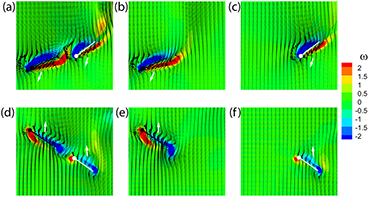
To probe how the WWI influences the aerodynamic performance of the wings, we plotted the vorticity contours (figure 11), superimposed by the velocity vector field, for the ALL case as well as the FO and HO cases, at the instants where the maximum force enhancement/reduction was observed during takeoff. Figure 11 compares vorticity and velocity vector fields of the ALL, FO, and HO cases, during DS (a)–(c) and US (d)–(f). The close proximity of the wings, during both DS and US, is beneficial to the aerodynamic performance of the forewings due to the favorable distortion of the forewing's downwash caused by the interaction between the hindwing's LEV and the forewing's trailing edge vortex (TEV). The upward jet (which is downward in US) induced between this vortex pair reduces forewing's downwash. This effect is known as the wall or ground effect [46, 47]. On the other hand, in DS, the hindwing is in the wake of the forewing and is therefore negatively affected by the forewing's downwash. During the upstroke, the relative spacing of the wings and the direction of their motions is in such way that the hindwing is no longer directly in the wake of forewing and therefore the adverse influence of the forewing's downwash is minimal. In addition, the hindwing benefits now from a similar wall effect as the forewing and its performance is enhanced.
Figure 11. Vortical structures during wing-wing interaction. This figure shows a 2D slice with the vorticity contours (similar to figure 8(a), superimposed by the velocity vector field, for the ALL case ((a) and (d)) as well as the FO ((b) and (e)) and HO ((c) and (f)) cases, at the instants where the maximum force enhancement/reduction was observed. The slice is cut at 0.3R to capture both the FW and HW at close proximity. The FW and HW are depicted as black and white lollipop figures respectively. The white arrow represent the direction of motion of the wing. (a)–(c) are captured at t/T = 0.42 and (d)–(f) at t/T = 0.80 based on the forewings timing.
Download figure:
Standard image High-resolution image
The vertical forces were not substantial in the upstroke phase but the horizontal forces were. We found that both the FW (8.8% decrease in 2nd US, 40% decrease in 3rd US) and HW (14.6% decrease in 2nd US, 7.3% decrease in 3rd US) horizontal forces were negatively affected by interaction.
4. Concluding remarks
To accomplish a takeoff which lasts only as long as a portion of a wingbeat, the damselfly generates large aerodynamic forces in both downstroke and upstroke. The kinematics of all four wings are carefully manipulated and controlled. While the damselfly can modulate the kinematics of each one of the four wings independently [23], our measurements show that these changes are also interdependent (i.e. via phase relationship). In the takeoff wingbeat, the damselfly manipulates both the average pitch angle as well as the twist angles of the wing causing the formation of a stable leading edge vortex which stays attached to the wing throughout the translation phase of the wing motion, during both down and up strokes. In the following flapping strokes, when the insect transitions to forward flight, the angle of attack is substantially reduced in the upstroke. Consequently, the LEV formation in the upstroke is almost completely inhibited and the magnitude of the aerodynamic forces attenuates accordingly.
Current literature indicates that the downstroke generates 80% of the total force during forward flight of Cicadas [38], 50–100% total vertical force in bumblebees as flight speed increases from 1–4 m s−1 [48], and 75% of total force for damselflies in forward flight [12]. The upstroke seems to contribute minimally to force generation but could be useful in thrust generation which is usually about 10–20% of bodyweight; a meager amount [26]. However, when flight mode demands an extra boost of force, the upstroke may become active such as during hovering or flight initiation [49, 50]. Our measurements and analysis in this study shows that the damselfly can actively change the aerodynamic role of the upstroke in generating aerodynamic forces as small as only a portion of the body weight to as large as few times the body weight. The primary factor responsible for high forces in the US during takeoff was the LEV observed on the wing surface (see figure 7). This LEV was present on both the fore and hindwings contrary to previous studies on free flight of four-winged fliers [19, 23]. The presence of the LEV produced the extra pressure difference on the wing as shown in figure 8, which is responsible for amplifying the forces on the wings. Our results indicate that the LEV boosted the pressure difference in the first upstroke by as much as 220% compared to other strokes, as the wings in all strokes flapped with similar velocities in the US.
Furthermore, when taking off, the damselfly flaps its fore and hind wing with a carefully selected phase difference where the forewings lead the hindwings by a small phase. Our results show that the effect of wing-wing interaction on the aerodynamic performance depends on both the phase difference and the relative orientation and location of the wings in space. Close proximity of the hindwing to the TEV of the forewing was shown to be beneficial to the forewing's aerodynamic performance via the so-called wall effect, in both DS and US. In addition, we found that the hindwing can also benefit from the wing-wing interaction, when lagging behind the forewing, if the orientation and spacing of the stroke planes are carefully adjusted.
Finally, in comparison to the non-jumping flights of other insects, the takeoff of damselfly is significantly faster when measured in wingbeat time, lasting only a wingbeat. The closet data we found in the literature belonged to the non-jumping takeoff of Rhinoceros beetle, which is also a four-winged insect. In the flight of the beetle, liftoff occurred within 3 WB [9]. Nevertheless, unlike the damselfly there were no drastic changes in stroke amplitude and AOA leading up to takeoff stroke. In addition, the fore and hindwings bore the burden of force generation equally in damselfly takeoff, whereas in beetle takeoff, most of the forces were generated by the hindwings. In both non-jumping takeoffs of the damselfly and beetle, however, the horizontal distance covered during takeoff was greater the than vertical displacement of Center of Mass (CoM) and after liftoff, the stroke planes with respect to the horizon were drastically reduced as the insect attained a horizontal posture.
Acknowledgments
The authors gratefully acknowledge support from National Science Foundation (grant number CBET-1313217) and Air Force Research Laboratory (grant number FA9550-12-1-007) monitored by Dr Douglas Smith.