

Abstract
The visual cue of optical flow plays an important role in the navigation of flying insects, and is increasingly studied for use by small flying robots as well. A major problem is that successful optical flow control seems to require distance estimates, while optical flow is known to provide only the ratio of velocity to distance. In this article, a novel, stability-based strategy is proposed for monocular distance estimation, relying on optical flow maneuvers and knowledge of the control inputs (efference copies). It is shown analytically that given a fixed control gain, the stability of a constant divergence control loop only depends on the distance to the approached surface. At close distances, the control loop starts to exhibit self-induced oscillations. The robot can detect these oscillations and hence be aware of the distance to the surface. The proposed stability-based strategy for estimating distances has two main attractive characteristics. First, self-induced oscillations can be detected robustly by the robot and are hardly influenced by wind. Second, the distance can be estimated during a zero divergence maneuver, i.e., around hover. The stability-based strategy is implemented and tested both in simulation and on board a Parrot AR drone 2.0. It is shown that the strategy can be used to: (1) trigger a final approach response during a constant divergence landing with fixed gain, (2) estimate the distance in hover, and (3) estimate distances during an entire landing if the robot uses adaptive gain control to continuously stay on the 'edge of oscillation.'
Export citation and abstract BibTeX RIS

Content from this work may be used under the terms of the Creative Commons Attribution 3.0 licence. Any further distribution of this work must maintain attribution to the author(s) and the title of the work, journal citation and DOI.
1. Introduction
A major challenge in robotics is to achieve autonomous operation of tiny flying robots such as 25 g 'pocket drones' [11] or more extremely the 80 mg Robobee [33]. Flying insects provide a rich source of inspiration for solving this challenge, since they are able to navigate successfully on the basis of a very limited sensory and processing apparatus. Flying insects rely heavily on optical flow, i.e. the apparent motion of world points caused by the relative motion between the observer and the environment [21]. Also for robots this cue is promising as it can be extracted from a single passive camera, implying light weight and relatively little energy consumption [14, 16, 18, 41].
It is well known that optical flow conveys information on the ratio between distance and velocity, and that additional information is necessary to disentangle these quantities. This 'scaling' can be performed by means of maneuvers that have a known range or velocity (as in parallax [29]), or with any sensor that directly or indirectly provides information on the (change in) distance or velocity estimates, e.g. accelerometers or sonar [12, 32]. Interestingly, flying insects such as fruit flies do not seem to have scaling sensors [15]. In addition, it is unlikely that they know the range of their maneuvers since they only have access to their air speed, not their ground speed [6].
Still, flying insects are able to navigate successfully. The key to this success is that flying insects follow straightforward strategies based on optical flow observables. First, it was found that honeybees keep ventral flow (defined as  ) constant when they perform grazing landings [42]. This strategy was studied for flying robots and simulated spacecraft [27, 35, 37, 45]. However, these studies required a 'pitching' law, ultimately depending on an estimate of the height and velocity. The main reason seemed to be the absence of control of the vertical dynamics. Therefore, more recent landing strategies also include the flow divergence (D, typically defined as
  , with the positive z, vz axis pointing up) or time-to-contact (
 ) [1, 24, 26, 28]. These strategies either enforce a decreasing time-to-contact (as humans do for car braking [30]) or keep the divergence constant (as honeybees do for straight landings [3]). Recently, in [15], ventral flow and divergence were combined with slope estimation and an anemometer in order to fly over uneven terrain, without a need for inertial frames or scaling sensors.
The absence of velocity and distance information has been a defining property of the work on optical flow-based navigation strategies. However, the following observations suggest that for successful navigation distance estimates are still of importance. First, flying insects do seem to have distance-dependent behaviors. For instance, van Breugel et al [6] remarked that fruit flies extend their legs at a specific distance from an oncoming object. Second, for successful optical flow landing control, the gains of the controller are tuned to a range of specific heights and velocities. For instance, for the constantly decreasing time-to-contact landings in [9, 28], the gains are scheduled by means of τ, along a trajectory starting at a specific initial height and velocity. Third, while for a constantly decreasing time-to-contact landing it is possible to perform a final landing procedure (when the time-to-contact is almost zero), it is not obvious how such a procedure should be triggered in a constant time-to-contact or divergence landing.
It is actually possible to estimate distances based on optical flow, if a robot has access to copies of its control input signals (referred to as 'efference copies' in the biological literature). Two main strategies have been proposed so far in the literature.
The first strategy for estimating distances is well-established in the field of image based visual servoing (IBVS). In the task of IBVS a robot has to regulate certain target features to desired image locations, without knowing a priori their dimensions or geometry. Quite early it was observed that if a fixed gain is used to map an image error to a control input, the response of the system depends on the distance to the target [8]. Given a model of the robot's dynamics, the effects of the robot's actions on the image features can be used to estimate the distance to the target (e.g. with a nonlinear observer). The distance estimates allow for smooth control in an adaptive gain control scheme [2].
The second strategy for estimating distances was recently proposed by [6]. They showed that during a constant divergence approach of an object, the control input u (the thrust) is proportional to the distance d, and that efference copies can then be used as a stand-in for distance. This solution was tested on a camera mounted on a rail and successful distance estimates were obtained by integrating information during the entire approach.
Both strategies above assume that the robot's accelerations are completely determined by the control inputs. However, flying robots and insects are also subject to significant external accelerations caused by wind or wind gusts.
The main contribution of this article is the proposition of a novel, stability-based, strategy for distance estimation with optical flow and efference copies. The central idea is to estimate distance by exploiting the self-induced oscillations that result from the fundamental imperfection of fixed-gain optical flow-based control. The distance estimation strategy provides two major advantages with respect to the previously proposed strategies: (1) it works straightforwardly even in the presence of wind, and (2) it can be used in a broader range of maneuvers, and notably in hover.
The remainder of the article is organized as follows. In section 2, we introduce the notations used in this article and discuss the intrinsics of a constant divergence landing. Subsequently, the new stability-based strategy to distance estimation is proposed in section 3. In section 4 it is shown how self-induced oscillations can be used to trigger a final landing procedure. Subsequently, in section 5 adaptive gain control is introduced to determine the distance in hover and to estimate distances along an entire constant divergence landing. In section 6, the findings are empirically verified with real-world experiments using a Parrot AR drone. Finally, the results are discussed in section 7 and conclusions are drawn in section 8.
2. Constant divergence landing
The novel distance estimation strategy will be studied in the context of a landing task. In this section, the main aspects of a constant divergence landing are explained. Figure 1 shows the definition of the axes as used in the formulas. In order to keep the equations as uncluttered as possible, most of the analysis in this article focuses purely on the z-axis. Generalizations to other looking and movement directions are easily made (see, e.g., appendix

Figure 1. Axis system employed in the article. The bottom camera on the robot looks straight down and perceives the ground surface. When descending, a diverging flow field is perceived in the camera view, allowing the robot to determine the divergence  .
.
Download figure:
Standard image High-resolution imageThe robot perceives an optical flow field  in its bottom camera view. The divergence is defined here as:
  , which is equal to
  if the robot is looking straight down. In this article as 'visual observable' the variable
  is used, which is the relative velocity
  . Hence, a constant or zero divergence maneuver is also a constant or zero
  maneuver.
If the robot lands while keeping  constant, the height and vertical velocity will obey the formulas:


which with a negative initial velocity vz0 has vz and z simultaneously converge to 0, 
3. Instability of constant divergence landings
The onset of the work in this article came from the difficulty of making optical flow-based landing strategies work on real micro air vehicles (MAVs). The study in [28] is especially instructive, since multiple control laws are studied, of which the gains depend to different extents on the initial height and velocity. Especially important are the remarks and observations on the difficulty of getting the optical flow control to work close to the landing surface, where oscillations tend to occur. It is even suggested to disengage the optical flow control under a threshold distance (as is also done in [45]).
Please note that it is not easy to identify the cause of oscillations close to the surface when performing vision-based control with a real MAV. Oscillations close to the ground can potentially be explained by the 'ground effect' due to the MAV's downwash and by the vision process (more blurry images, larger optical flow vectors that are harder to track). Below it will become clear though that even without such additional effects, the instability problem arises.
Based on the dependence of the gains on the actual height and velocity, in this article a novel strategy is proposed for distance estimation: stability-based distance estimation. In this section, first the fundamental reason for the gain tuning problem of optical flow based control is explained (section 3.1). Subsequently, a specific control law is assumed and it is shown analytically that the stability directly relates the control gain to the height (section 3.2).
3.1. Fundamental reason for gain tuning
Before going into why a single gain is only stable for a given range of heights, first the equations of motion will be described. Let us start with the model in [6]. In the notation of a state space model:

where the state vector ![${\bf{x}}={[z(t),{v}_{z}(t)]}^{T}$](https://content.cld.iop.org/journals/1748-3190/11/1/016004/revision1/bbaa0b98ieqn12.gif) , and
, and  , so that:

This model assumes that uz = az, which effectively implies that any possible gravity is subsumed under the uz-term:

where  is the actual upward thrust generated by the robot in Newton. It is common in control system theory to subsume factors such as gravity and the mass into uz, as the calculation of
  is straightforward and does not depend on any state variables.
Equation (5) is only valid if the control force is the only force acting on the robot. In a vacuum environment this can be approximately correct, e.g. for a moon landing. However, a robot flying in the air will undergo additional accelerations. Therefore, in this article, the drag force will be modeled, which depends on the robot's movement relative to the air:

where:

and  indicates the directionality of fD along the z-axis. This leads to an additional acceleration:

in which fD is a time-varying value involving a non-linear function of vz and an uncontrolled variable  .
.
Now, let us start from the visual observable  :
:

If  is differentiated over time, it results in:

Using equation (9):

Assuming az as in equation (8):

Differentiating this formula with respect to  gives:

Equation (13) shows that a change in thrust has a larger effect on the change in  closer to the landing surface than far away (independently of external accelerations)1
Thus, a control gain for regulating
closer to the landing surface than far away (independently of external accelerations)1
Thus, a control gain for regulating  that leads to a satisfactory control performance far away from the landing surface, will lead to very large effects on
  and hence indirectly on
  close to the landing surface. Although theoretically one could use
  directly for distance estimation (
 ), in practice this value is extremely noisy, since it involves a partial derivative with the noisy value
  .
.
3.2. Relation between control stability, gain, and height
In this subsection, it will be shown that the larger influence of uz on  at lower heights eventually leads to instability at a specific height. For the analysis, the following constant divergence control law is studied, using just a proportional gain Kz as in [6]:

where it is easy to see that in a noiseless, delayless system:

and hence  . Real systems always have some noise and delay. Below, it will be shown that just discretizing the control with zero-order-hold (ZOH) will already introduce an instability into the system.
Let us assume the state space model of equation (4), ignoring drag for the moment. The corresponding observation is:

which is a nonlinear function. Linearizing the state space model gives:

so that the state space model matrices are:

As mentioned, the continuous system without noise and delay is stable (equation (15)). Here, the discretized system is studied, which has the following state space model matrices corresponding to the continuous ones in equation (18):

where T is the discrete time step in seconds. The transfer function of the open loop system can be determined to be:


where we use w as the Z-transform variable, since z already represents height. The feedback transfer function is:

Equation (22) shows that, given a gain Kz and time step T, the dynamics and stability of the system depend both on the height z and velocity vz.
Figure 2 is the root locus plot of G(w). For the Z-transform any pole in the unit circle is a stable pole. The different elements of the plot can be found back in equation (22). The numerator indicates a single finite zero at:

Given  ,
,  , and
, and  , w0 is positive and due to the typically small T values slightly smaller than 1. There is also a negative infinite zero. Since the denominator of equation (22) is a second order equation in w, G(w) has two poles, both of which are stable. For Kz = 0, the poles are located at w = 1. As the gain Kz increases, one pole moves toward the finite zero and one toward the infinitely negative zero. This latter pole is interesting, because as soon as it passes
  , the system becomes unstable. Setting
  in the denominator and equating it with 0 gives an equation for the unstable gain value Kz:


Figure 2. Root locus plots of a ZOH-model with  for z = 1 m and z = 10 m. The plots are equal in shape, but for each point Kz is different. This is indicated for the (approximations to) the values of Kz at which the system becomes unstable (
 ).
).
Download figure:
Standard image High-resolution imageThis implies that given a specific gain Kz and time step T, there is always a height at which the control system will become unstable:

When using a fixed gain, a tradeoff has to be made between the control performance at a larger height (requiring a large gain) and at lower heights (requiring a small gain). Please remark that the instability at lower altitudes is exactly what is observed for robotic systems performing constant divergence landings!
3.3. Including wind
In this subsection it is shown that also for a model with wind, the instability of the system given a Kz depends on z. Including wind leads to a changed formula for  (see equations (6) and (8)):

where from now on β will stand in for the constant  . In order to obtain a linear state space model, this equation is linearized to obtain:

where the factor multiplied with  is a constant in the linearized model (
 and vz are given the values at the linearization point). In order to avoid cluttering the formulas, this constant is represented by
  (where
  ). This leads to the following continuous, linear state space model:

which results in the Z-transform matrices:


and a rather involved transfer function H(w). The root locus plot of H(w) is very similar to that of G(w), also with a negative infinite zero. Following the same procedure as for the 'vacuum' model, setting  and equating the denominator with 0, gives:

Equation (32) includes many instances of p that depend on vz and  , and also contains a term in the denominator with vz. This suggests that there is no fixed linear relation between Kz and z. However, closer inspection shows that the term
  . Rearranging terms, this leads to:

which still depends on p. It turns out that the fraction that is multiplied with z is almost identical to the fraction  . Indeed, solving equation (32) for different variable settings gives almost identical results to equation (24).
3.4. Continuous system with drag and delay
The previous subsections discussed discretized models for which unstable Kz exists, and where the limit case can be analytically expressed as a function of z. In order to show that continuous systems encounter the same type of phenomenon, figure 3 shows the root locus plot of a continuous system with wind, a delay of  and
and  . The delay introduces two zeros in the (unstable) right-hand plane of this continuous root locus plot. A few values of Kz are plotted, where the poles get an imaginary component and where they cross the imaginary axis (shown for z = 10 m and z = 1 m).

Figure 3. Root locus plots of a continuous model with a delay of  (as approximated by a second order Padé transfer function), and aerodynamic drag with
  , for z = 1 m and z = 10 m. The plots at different heights are equal in shape, but for each point in the plot Kz is different. This is indicated for the (approximations to) the values of Kz at which the poles get an imaginary component (start of oscillations), and where they cross the imaginary axis (become unstable).
Download figure:
Standard image High-resolution image4. Stability-based distance estimation
In the previous section, it was established that the instability of a constant divergence approach system depends on the distance. If this instability can be detected by a robot or insect, it can be used for distance estimation!
4.1. Detection of self-induced oscillations
The instability discussed in section 3.2 is induced by the robot itself. Before the system gets unstable, it will start to show oscillations. This can be seen for instance in figure 3. When Kz = 24.3, the control system's poles will start to have an imaginary component and hence oscillate around the desired value from z = 10 m downward. In the field of aerospace, such self-induced oscillations are a well-known problem, and referred to as pilot-induced oscillations (PIO).
The two most important properties of self-induced oscillations are that (1) there is a phase shift between the observations and control inputs in the order of 90–180◦, and (2) the oscillations are of a significant magnitude. Let us have a look at a simulated landing to see how this phenomenon occurs for the studied constant divergence landings. For the simulations, a ZOH-model is assumed with a time step T = 0.03 s,  , a mass of 1 kg, and a delay of
  (as in section 3.4)2
. The left part of figure 4 shows a landing for Kz = 20,
(as in section 3.4)2
. The left part of figure 4 shows a landing for Kz = 20,  ,
,  ,
,  , in wind still conditions (
 ). It shows that the landing goes smoothly, until the very end at
  at which point the robot's height starts to oscillate.

Figure 4. Left: landing in simulation with  . The red line is the height, the black line is the point at which the onset of oscillations is detected with the robot's observables. Right: some of the main relevant variables: the true relative velocity
  (dark yellow, dashed), the estimated relative velocity
  (magenta, solid), the thrust
  (blue, dotted), and the windowed covariance
  (black, dashed) and
  (black, solid).
Download figure:
Standard image High-resolution imageThe right part of figure 4 shows the main relevant variables, zooming in at the few seconds before landing (until t = 26 s the variables do not vary much). The dark yellow dashed line is the ground-truth  , while the magenta solid line is its delayed version
  as observed by the robot. The blue dotted line represents the thrust
  . Toward the end of the landing
  starts deviating significantly from its reference point −0.1 (indicated with the thin dotted magenta line). It even obtains positive values, which means that the robot goes up. This itself could be used for the detection of instability, were it not that a wind gust can also move the robot upward, causing a positive
  at a larger height. The problem here is that the effects of the thrust changes have an ever larger and quicker effect on the relative velocity when getting closer to the landing surface. This response will get so quick that the robot starts getting in resonance with its own delay, as testified by the phase shift between
  and
and  . The robot starts thrusting up while going up and thrusting down while going down.
The two properties of self-induced oscillations (phase shift and magnitude) can be captured with the covariance between the ground-truth  and the thrust
  . The right part of figure 4 shows
  as determined over a window of the last W = 20 time steps (black dashed line):

During the smooth part of the trajectory  is a small negative number: when the robot descends too fast (
 too negative) the robot thrusts more up, and vice versa. Towards the end of the landing the observable
  starts to change too quickly for the control system and
  becomes positive: if the robot descends too fast (
 too negative) the robot will thrust less up, and thus it starts inducing oscillations.
How can robots detect self-induced oscillations without access to the ground truth  ? There have been several investigations on the automatic, on board detection of self-induced oscillations [7, 10, 34, 38, 47]. A typical detection method involves a fast Fourier transform (FFT) of the observations [7, 38], looking for the specific frequency band related to the self-induced oscillations. In this article, in the interest of a computationally efficient and straightforward method, we will investigate the use of the
  as a proxy for
  . In figure 4,
  is shown with a black solid line. It is always negative, as
  , and hence mostly captures the magnitude of the oscillations. The
  can be used in conjunction with
  for detecting the onset of oscillations. The black line in the left part of figure 4 shows the first point during the landing at which
  and
and  .
.
In order to test the hypothesis that the onset of oscillations is related to the magnitude of the gain and the height of the robot, simulation runs were performed for gains  and for various types of wind
  m/s. Furthermore,
  ,
,  ,
,  . The left part of figure 5 shows the results of this experiment, with the different Kz on the x-axis and the corresponding z at which self-induced oscillations are detected on the y-axis. Each Kz additionally is represented with a different marker, and the markers are colored according to the wind velocity, from blue (−3 m/s) to red (3 m/s). The black dashed line is a linear least-squares fit through the points, with parameters
  .
.

Figure 5. Left: oscillation detection heights for different gains Kz for different wind velocities. The color of the marker represents the wind velocity, ranging from −3 m/s (blue) to 3 m/s (red). The black dashed line is a linear fit through the detection heights. Right: results for experiments with a PI-controller, with Iz = 1 as the I-gain.
Download figure:
Standard image High-resolution imageThere are three main observations. First, as the linear fit shows, higher gains result in oscillations further away from the landing surface. Hence, a fixed gain will result in self-induced oscillations around a certain height. The detection of these oscillations can be used for instance for triggering landing responses (such as the leg extension by fruitflies). Second, a considerable wind difference between −3 to 3 m/s leads to a relatively small (for MAVs) difference of  in the height at which self-induced oscillations occur. Third, the colors show that there is a slight correlation between the detection height and the wind velocity. Analyzing the landings with wind shows that for the higher wind velocities, the control system has more difficulties tracking
  , leading to a steady-state error. This suggests that introducing an integrator term could resolve this problem. The results of a PI-controller, with Kz as the P-gain and Iz = 1 as the I-gain, are shown in the right part of figure 4. Since the PI-controller can cancel the steady-state error, the reference
  is tracked much better. As expected, self-induced oscillations still occur, and the detection heights are much closer together. Moreover, inspection of the marker colors shows that there is no obvious relation anymore between the wind velocity and the detection height. In order to keep in line with the system that was analyzed theoretically, for the remainder of the article we will focus on the P-controller setup with gain Kz.
4.2. Wind gusts and actuator efficiency
In the previous subsection, the feasibility of detecting self-induced oscillations for distance estimation was shown. However, two factors were not modeled that could have a significant influence on the practicality of the approach.
First, during a typical landing outdoors the wind is not constant. The wind can vary and sudden wind gusts can occur. In the simulation, wind gusts are added to the simulation in the form of a sine function:

where W determines the magnitude of the gusts and a the period.
Second, it is unlikely that a robot's command signal (and hence efference copy) is equal to  . A command signal
  (in any unit, e.g. the commanded RPM of a robot's propellors or the flapping frequency of an insect) is related to
  (in Newton) with an actuator effectiveness function:
  . In flying robots such as rotorcraft or flapping wing vehicles the function f, in turn, depends on the air flow. Here, a rotorcraft is assumed and the relation between actuator effectiveness and air flow is modeled according to findings on propellors in [44]. Specifically, the following formula was used:

so that both the offset and slope of the efficiency change over different air velocities.
The left part of figure 6 shows a landing with a rather extreme scenario, in which the average wind velocity is 0 m/s, W = 4, a = 1, b = 0.5, and c = 0.5. This means that per every π seconds, the wind varies from −4 to 4 m/s! The red line in the figure is the height over time, the black line indicates the height at which self-induced oscillations are detected. The right part shows the results over many landings with the same settings but different wind velocities, from −3 m/s (blue) to 3 m/s (red), to which the gusts are added during each landing. The black dashed line is a linear fit through all the detection heights for all gains Kz.

Figure 6. Left: landing in gusty wind conditions (ranging from −4 to 4 m/s in π seconds. The red line is the height over time, the black line the detection height. Right: oscillation detection heights for different gains Kz for different wind velocities in gusty wind conditions. The color of the marker represents the wind velocity, ranging from −3 m/s (blue) to 3 m/s (red). The black dashed line is a linear fit through the detection heights.
Download figure:
Standard image High-resolution imageThe results show that despite the very gusty conditions and varying actuator efficiency, there is still a positive linear relation between z and Kz. The uncertainty is slightly higher though than for a constant wind and actuator efficiency, especially for larger gains/heights. It is important to emphasize that the actuator efficiency function f does not have to be known. Assuming a linear actuator efficiency function and using that the fit should pass through  , a single landing with a fixed gain in principle suffices to 'calibrate' the linear relation between z and Kz.
5. Adaptive gain control
5.1. Distance estimation in hover
In principle, the detection of self-induced oscillations could be sufficient for flying robots (or insects) to determine when they are close to their landing target. This allows for the triggering of a final landing procedure and hence is behaviorally very relevant. However, it would be extremely useful if the robot could determine height at any distance to the landing surface.
Surprisingly, the proposed stability-based strategy for height estimation does not require the robot to land! Equation (25) (derived for the vacuum condition) does not depend on vz, nor on c2. This suggests a strategy for determining the height around hover: the robot can set  and change its gain Kz so that the control loop starts exhibiting small self-induced oscillations. The gain at such a point is then a stand-in for the height.
Specifically, a control law can regulate  by continuously adapting the gain Kz. This leads to the following adaptive gain control setup. An inner loop uses
  , while an additional outer loop controls Kz:


where ![$P,I\in [0,1]$](https://content.cld.iop.org/journals/1748-3190/11/1/016004/revision1/bbaa0b98ieqn106.gif) are a proportional and integral gain for the outer loop control, both relative to the current
are a proportional and integral gain for the outer loop control, both relative to the current  . The reason for this is that larger heights involve higher speeds, so that Kz should be changed more quickly for larger
  than for smaller
  . The adaptive gain control is represented as a control diagram in figure 7.

Figure 7. Control diagram of the proposed adaptive gain control strategy.
Download figure:
Standard image High-resolution imageThis strategy has been tested in simulation for  and
and  . The simulation stops when
  . Figure 8 shows for each simulation run the last gain and height with a marker. The markers are again color-coded for the wind from blue (−1 m/s) to red (1 m/s). The black dashed line shows a linear least squares fit.

Figure 8. Results of simulated hover tests. The robot is placed at different heights with Kz = 10 with  . The gain is then adapted with
  . The x-markers show the height z and Kz at the first time instant in which
  . The markers are color-coded for the wind (blue = −3, red = 3). The black dashed line is a linear fit.
Download figure:
Standard image High-resolution imageThe main result is that this method indeed gives an approximately linear relationship between z and Kz, with linear fit  . Although the wind influences the hover altitude (since it is not accounted for in the initial thrust) it again hardly influences the results.
5.2. Distance estimation during landing
Is there a possibility of landing and continuously estimating the distance to the surface? Figure 8 suggests that there is. If the robot descends while keeping  at a fixed negative value, then the gain Kz will directly represent the height z during the landing. This strategy of 'landing on the edge of oscillation' can use the exact same adaptive gain control as explained above, but then with
  .
.
Simulations of this strategy have been performed for  . The implementation of the strategy starts with a hover maneuver (
 ) with Kz = 50, I = 0.005, and P = 0.15. If in hover the condition
  is met, the landing is commenced. During landing
  ,
,  .
.
Figure 9 shows the Kz versus z during the landing phase. The markers are color-coded for the starting height z0 in the landing phase, from blue (10 m) to green (5 m). Each starting point is indicated with a red cross. After switching from  to
to  , it takes some time for the outer loop to compensate, which causes Kz to vary at the start of the landing phase. After that, all Kz are linearly related to z, with linear fit
  .
.

Figure 9. Results of simulated tests landing on the edge of oscillation. The robot is placed at different heights with Kz = 50. Then, it starts adaptive gain control with  . First
  , and when for the first time
  , the relative velocity set point is changed to
  .
.
Download figure:
Standard image High-resolution image6. Real-world experiments
In this section, experiments will be performed with a Parrot AR drone in order to verify the main findings from the theoretical analysis and simulations in the previous sections.
6.1. Experimental setup
The experimental setup is shown in figure 10. A Parrot AR drone 2.0 is used, running the Paparazzi open source autopilot software on board [22, 36]3 . This means that the Paparazzi autopilot is in full control of the AR drone, processing the sensors on board. The AR drone is equipped with an IMU (accelerometers, gyros, magnetometer, pressure sensor), and a downward pointing camera and sonar. For the purpose of the experiments, the vertical control loop implements the fixed and adaptive gain controls explained in the previous sections, and hence only uses the relative velocity estimates coming from the vision process, which is further explained below. The sonar is logged for analysis purposes. The horizontal position is stabilized as much as possible. In the indoor experiments, an Optitrack motion tracking system measures the drone's X- and Y-position at 120 Hz with millimeter precision. Paparazzi then performs the outer loop control on the basis of these measurements. In the outdoor experiments, where the drone is subject to much larger disturbances from the wind, a human pilot attempts to keep the drone in the same horizontal position by means of manual control.
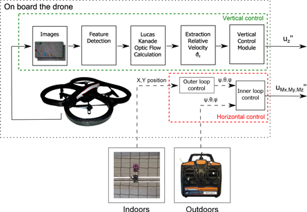
Figure 10. Experimental setup. The Paparazzi open source autopilot [22, 36] runs on board the Parrot AR drone 2.0, processing the images on board for the autonomous vertical control loop. The horizontal control loop is not relevant to the current experiments and relies on position estimates from a motion tracking system in the indoor experiments and on manual control inputs in the outdoor experiments.
Download figure:
Standard image High-resolution imageThe vision process is designed as follows. The images are processed with a rather standard vision pipeline available in Paparazzi. Maximally 40 corners are detected with the method in [40], and these corners are tracked to the next image with the Lucas–Kanade optical flow algorithm [31]. The optical flow divergence is estimated by means of the distances between tracked corners in two subsequent images. From all possible pairs of optical flow vectors, 50 pairs are sampled with replacement. Per pair of optical flow vectors, the image distance in the previous image  and the image distance in the current image dt (see figure 11) are used for a single estimate i of the divergence:

A global divergence estimate  is obtained by taking the median of estimates Di,
  . With the help of the frame rate (which is on average 25 Hz) and the camera's field of view (
 in the horizontal direction), this estimated divergence is transformed to the estimate of the
  expressed in
  .
.

Figure 11. Illustration of the image distances  (red) and dt (green) for a single pair of selected optic flow vectors (black vectors). A single pair of vectors gives rise to a single estimate of the optical flow divergence, Di, by means of equation (39).
Download figure:
Standard image High-resolution imageThe estimated relative velocity  is low-pass filtered over time and then used in a control loop
  , where
  is the vertical thrust command. Please note that in the real-world experiments, the thrust command is bounded to the interval
 ![${u}_{z}^{\prime }\in [0.6\;M,0.9\;M]$](https://content.cld.iop.org/journals/1748-3190/11/1/016004/revision1/bbaa0b98ieqn141.gif) , where M is the maximal thrust that can be commanded to the propellors. The program allows both fixed gain control and adaptive gain control as in section 5.2. Experiments were performed in an indoor and an outdoor environment, shown in figure 12. The main parameters used in the experiments have been determined empirically for the used AR drone 2.0 and will be mentioned along with the relevant experiment.
, where M is the maximal thrust that can be commanded to the propellors. The program allows both fixed gain control and adaptive gain control as in section 5.2. Experiments were performed in an indoor and an outdoor environment, shown in figure 12. The main parameters used in the experiments have been determined empirically for the used AR drone 2.0 and will be mentioned along with the relevant experiment.

Figure 12. Left: indoor test environment. Right: outdoor test environment.
Download figure:
Standard image High-resolution image6.2. Indoor experiments
First, it is verified that a fixed-gain constant divergence landing results in instability at different heights. The results of this test for  (green, blue, and red lines) and
  are shown in figure 13. The left plot shows the height over time for nine such landings. Dotted lines indicate the first point at which
  , set to trigger the drone's automatic landing procedure. This value is larger than in simulation to prevent too-early landing triggering. The reason is that the real drone does not only have a delay in the observations, but also noise and it is subject to larger disturbances and uncertainty in the actuation. The main observation from the figure is that also for the real robot, higher gains lead to an instability at larger heights. The right part of figure 13 shows a marker for each point
  at which self-induced oscillations are detected, and a corresponding linear fit, with parameters
  . The mean absolute error when using this function for height estimation is 0.11 m.

Figure 13. Left: nine fixed-gain constant divergence landings of a Parrot AR drone, with set point  and gains
  (green, blue, and red lines, respectively). The inset shows the drone in the indoor environment. The dotted lines show the first point at which
  indicating the onset of self-induced oscillations. Right: per landing, a marker is shown for the point
  at which self-induced oscillations are detected. The dashed black line is a linear fit through these points.
Download figure:
Standard image High-resolution imageThe second finding to verify is the determination of height around hover. For the real robot,  is employed, with I = 0.25 and P = 10. During the hover experiment, the robot has been sent to different heights, subsequently activating the adaptive gain control. In order to get an impression of what the adaptive control does, let us first zoom in on the relevant variables during a short part of the flight, shown in figure 14. In this part of the flight, the drone has just ascended to ∼2 m (see top left plot), while it has an initial gain of Kz = 1.0 (bottom left). The drone starts to regulate its relative velocity to
  (top right), and initially there are no self-induced oscillations as witnessed by the
  (bottom right). The low covariance makes the gain
  increase over time. This gradually causes
  to show ever larger oscillations, which leads to more negative
  . Around t = 114.5 s, the covariance reaches and overshoots its set point, and the gain
  starts stabilizing around 1.6 in order to keep the covariance around −0.025. The question now is at what values
  will stabilize at other heights, and whether there is indeed a linear relationship between z and Kz.

Figure 14. Signals during a small part of the indoor hover experiment. Top left: the height over time. Top right: relative velocity over time. The magenta line is the  used for control, as determined with computer vision, while the yellow line is the
  as calculated with the help of the Optitrack measurements (not used in control). Bottom left: the gain over time. The light green solid line is Kz, the dark green dashed line is
  (see equations (36) and (37)). Bottom right: the dashed–dotted line is the covariance of the control input
  and
and  , while the dotted line is the set point for the covariance (
 , see equation (38)).
Download figure:
Standard image High-resolution imageThe middle row of figure 15 shows the result of having the drone hover at different heights with  . The left plot shows a short time period during which the drone is continuously adjusting its gain (Kz and
  shown with the solid and dashed green lines, respectively), while attempting to keep the same height (z is represented by the red line). The right plot summarizes the results of five of such periods. The small blue markers represent the instantaneous
  -pairs, while each large red marker is the average
  over each period. The dashed line is a linear least squares fit through the red markers. Although more noisy than in simulation, the relation between z and Kz seems to be roughly linear, as predicted by the theoretical derivation. When using the linear fit
  as a height estimation function, the median absolute error of all observations is
  m, while the mean absolute error is 0.26 m.

Figure 15. Indoor results adaptive gain control. Top: photo during an indoor experiment. Middle row: results of hover experiments at different altitudes. Adaptive gain control is used with  . The left plot shows Kz,
  , and z over time for a short period at a specific height, the right plot summarizes the result over five such periods at different heights. Bottom row: results of landing on the edge of oscillation. The left plot shows Kz ,
  , and z over time for a single landing, while the right plot has markers for all
  -pairs of three such landings. See the text for further details.
Download figure:
Standard image High-resolution imageThe third finding to verify is the possibility to land on the edge of oscillation. The AR drone is sent to a height of 3.5 m. Then, the adaptive gain control is started, at first with  . As soon as
  , the landing phase starts. The bottom row of figure 15 shows the results for this test. The bottom left plot shows Kz,
  , and z over time during a single landing on the edge of oscillation. The right plot shows the points
  of this and two other landings, where different experiments have different markers and colors. The dashed line is a linear fit through all points. Although the results are quite noisy, again a roughly linear relation appears, with as linear fit
  . In this case, the median absolute error of all observations is
  m, while the mean absolute error is 0.29 m.
6.3. Outdoor experiments
Outdoor experiments have been performed to confirm that the method also works in an outdoor environment with wind and wind gusts. The right part of figure 12 shows the outdoor experimental setup. The ground surface consisted of small stones, which already provide ample texture. Some beach toys were added to the scene to also ensure visible texture at larger heights. The bottom left part of figure 16 shows the summary of the results from the hover experiment. Just as indoors, there is a roughly linear relationship between the height z as measured by the sonar and the gain Kz as determined with the adaptive gain control. The median and mean absolute errors in height of the fit are both 0.31 m. The bottom right part of figure 16 shows the results from three landings on the edge of oscillation, again showing higher gains at larger heights. The median absolute error in height of the fit is 0.32 m, the mean is 0.40 m.

Figure 16. Outdoor results adaptive gain control. Top: photo during an outdoor experiment. Bottom left: results of hover experiments at different altitudes, with  . Bottom right: results of landing on the edge of oscillation. The markers are
  -pairs during the landing, while Kz is regulated so that
  .
.
Download figure:
Standard image High-resolution imageVideos of some of the experiments can be seen at4 .
7. Discussion
7.1. Flying insects
The presented strategy forms a novel hypothesis on how flying insects such as fruitflies and honeybees can estimate distances, viz. by means of the detection of self-induced oscillations. In [6] a different, thrust-based strategy for distance estimation was introduced, and its implications for landing insects discussed. In part, the implications of these strategies overlap. They both explain how flying insects can trigger landing responses at a particular given distance, such as fruitflies that extend their legs just before landing (e.g. [5]). However, there is a significant difference in the strategies, which has its consequences for the explanation of flying insects' behavior. A few notable differences in this respect will be highlighted below.
A first difference is in the possible explanation of the hover phase honeybees exhibit just before touchdown [13]. The hover phase could in principle be explained as a maneuver that is triggered by a distance measurement, for instance by means of the thrust-based strategy of [6]. However, the proposed strategy suggests instead that the hover mode is an intrinsic property of optical flow control and is part of the distance estimation itself. As the honeybee gets closer to the surface, its control gain will start becoming too high. This will result in self-induced oscillations and lead to a situation of zero divergence, i.e. hover. In this light, it is interesting to remark the characteristic little 'bump' in the trajectory in figure 4. Similar bumps can be observed in figure 4 in [13] (for almost straight landings), and in figure 5 in [42] (for grazing landings).
A second difference is that the stability-based strategy explicitly allows for the observation that a visual stimulus itself can trigger the landing responses, even for tethered insects [4, 43]. The reason for this is that the strategy depends on the control stability and hence the system bandwidth. A standard way to measure the system bandwidth is to make a Bode plot that maps the system's frequency response. At too-high frequencies, the phase shift between the quickly changing observation and the subsequent control input will become larger and the magnitude of the control input lower. If the magnitude of the triggered control input is large enough, a purely visual stimulus may be detected as a self-induced oscillation.
7.2. Flying robots
Concerning flying robots, the novel proposed distance estimation strategy provides a novel way to perceive distances with a single vision sensor. This may turn out to be essential for tiny flying robots such as the Robobee [33], for which any type of sensor is a significant payload [20, 23, 39]. For slightly larger drones such as 25 g 'pocket drones' (e.g. [11]), the finding is also immediately relevant. For instance, currently the lightest, fully autonomously flying robot is the 20 g DelFly Explorer [46], which uses a 4 g stereo vision system with onboard processing to avoid obstacles in its environment. The proposed stability-based strategy to distance estimation may provide a bigger potential to even lighter, single-camera solutions, also for obstacle avoidance. In addition, it can provide scale to monocular navigation methods such as visual odometry [12, 17]. Even for MAVs on the order of ∼1 kg or larger, the method may still be useful. It allows us to estimate potentially large distances without compromising the MAVs' payload capability.
However, in order for stability-based distance estimation to live up to its potential, some issues need to be further investigated. The experiments have shown the strategy to work in an onboard processing scheme with a Parrot AR drone 2.0 with a median height estimation error in the order of ∼0.3 m. As a proof of concept this suffices, but it is desirable to improve the accuracy of the measurement. This seems quite possible by further improving both the inner loop divergence control (which now only involved a P-gain) and the outer loop adaptive control. Moreover, other, more reliable ways of detecting self-induced oscillations may be created. Such improvements could not only lead to more accurate distance estimates, but also to smoother divergence control. If high-performance, but smooth landing trajectories are the goal, the gain should always be slightly below the critical gain value leading to self-induced oscillations.
8. Conclusion
In this paper, a stability-based strategy has been proposed with which a robot can estimate distances only on the basis of efference copies and optical flow maneuvers. Theoretical analysis of linearized models has shown that there is a linear relation between the fixed gain and the height at which instability arises. This analysis has been verified in simulation (including non-linearities and disturbing factors such as wind gusts) and on a real robotic platform. It has been demonstrated that self-induced oscillations can be detected by the robot and used to (1) trigger a final landing procedure, (2) determine the height in hover, and (3) continuously determine the height during a constant divergence landing.
Acknowledgments
I would like to thank Christophe De Wagter, Hann Woei Ho, and Tobias Seidl for the interesting discussions and comments on earlier versions of the manuscript.
Appendix A: Influence of wind on thrust-based distance estimation
In the introduction, it is mentioned that the 'thrust'-based strategy of [6] does not take into account external accelerations. In this appendix, some insight is provided into the effects on the distance estimates when introducing external accelerations by wind.
Let us first re-arrange equation (11):

This expresses z in terms of 'observables' ( and its time derivative
  ), and the vertical acceleration az. Adding an accelerometer to the robot will allow for estimation of z (e.g. [25]). Besides the addition of the accelerometer, this method also requires the time derivative of
  , which typically induces a lot of noise in the observation.
In [6], the assumption is made that az = uz, so that equation (40) becomes:

In [6] it has been investigated what would happen if a perfectly constant divergence landing is performed,  and
and  (c2 to indicate that
  has a negative set point):

Equation (42) shows that during a perfect constant divergence landing, the thrust uz is a scaled version of the height. Hence, it can be used as a stand-in for the height. For this reason, the method is referred to in this article as a 'thrust-based' method.
It is informative to study the effect of drag and wind on the required  , when the robot follows a perfect constant divergence landing. In such a landing,
  at every point by definition. The acceleration resulting from drag and the required
  are calculated to match. Figure A1
shows the value of
are calculated to match. Figure A1
shows the value of  for a robot with assumed values of m = 1 kg,
  , and g = 9.81 m/s2. Furthermore, CD = 0.25, and A = 0.25, which are rather conservative values representing for instance a small quad rotor. The figure shows the thrust
  versus height z in different environmental conditions: vacuum (red solid line), wind still, i.e.,
  m/s (black dotted), in a downward wind of
  m/s (blue dashed), and in an upward wind of
  m/s (green, dashed–dotted).

Figure A1. Illustration of the effect of air drag and wind on the height estimation strategy proposed in [6]. Height z versus thrust  in different environmental conditions (see legend). Two black lines illustrate an estimation error when the wind is unknown. The lines indicate that the thrust with a downward wind of −1 m/s at z = 0 m corresponds to a thrust in a wind-still environment (0 m/s) at a height of
  .
.
Download figure:
Standard image High-resolution image
Three main observations can be made from figure A1: (1) the red solid line in a vacuum indeed indicates the derived linear relationship between uz and z, (2) in a wind-still environment, this relationship is nonlinear but invertible, and hence still as useful, and (3) adding a modest wind speed to the equation already makes significant differences to  . Two black lines indicate that the thrust with a downward wind of −1 at z = 0 m corresponds to a thrust in a wind-still environment at a height of
  m. The curve for a wind of 1 m/s does not even match that in a wind-still environment. Hence, even with a perfect constant divergence landing these differences distort the relationship between uz and z.
So, in order to retrieve the right uz-curve (see figure A1), the wind will have to be measured. Flying insects may be able to measure the air speed with their hairs [19], while robots can be equipped with an anemometer, as in [15]. Although measuring the air speed and deducing wind velocity is a possibility, this does not lead to an easy solution of the distance estimation problem. First and foremost, controlling a constant divergence landing in a real system means dealing with sensing and actuation delays, visual inaccuracies, and changing external factors such as wind gusts. Any real system will thus deviate from the perfect landing profile, leading to the necessity of command signal variation and hence a varying  . Indeed, this effect can be seen in the raw
  estimates in [6] for the camera-system mounted on a rail. In [6] they tackled this issue with a robust estimation scheme that integrates information during the entire approach. The problems are much worse though for a freely flying system, which is also subject to wind.
Appendix B: Generalization to other movement directions
In section 4 it was shown that given a gain Kz, the stability of the vertical control loop with  depends on the height z. In this appendix the case is studied in which the camera still looks down in the z-direction, but the movement is in the horizontal x-direction. The control is thus based on the relative velocity
  . It will first be shown that the finding also generalizes to such horizontal optical flow control (section B.1). The stability-based method then does not require vertical motion. Subsequently, a thrust-based method is investigated for horizontal motion (section B.2). The thrust-based method always requires both horizontal and vertical motion.
B.1. Stability-based method
Let us start from the observation:

Since both the horizontal and vertical axes are involved, the state space model will have four variables. Linearizing the state space model gives:

so that the state space model matrices are:

Again, the discretized system is studied, which has the following state space model matrices corresponding to the continuous ones in equation (45):

where T is the discrete time step in seconds. The transfer function of the open loop system can be determined to be:


where we use w as the Z-transform variable, since z already represents height. The feedback transfer function is:

Equation (49) shows that, given a gain Kx and time step T, the dynamics and stability of the system depend on the height z.
Setting  in the denominator and equating it with 0 gives:

which leads to an equation that expresses the height at which the control system will become unstable in terms of the unstable gain value Kx:

which is exactly the same formula as for the vertical movements studied in section 4.
B.2. Thrust-based method
It is instructive to also look at what a possible thrust-based method would look like for the horizontal motion direction. For this, let us again start from the observation  , which is differentiated over time:

leading to:

Equation (53) shows that the height can be estimated with the help of a horizontal accelerometer measurement and the observables  ,
,  , and the time derivative
  (as was done in [25]).
If the relative velocity  (sometimes referred to as 'ventral flow') is kept constant, then
  , and:

where in a vacuum environment, ax can be assumed to be ux. A constant ventral flow and divergence landing would then again lead to a way to estimate z, as ux is known and  and
and  can be assumed equal to constants.
Interestingly, also this horizontal motion case does not allow for distance estimation while staying at the same height ( ). The reason for this can be seen when rearranging equation (54):

which shows that  implies ax = 0. Indeed, if
  ,
,  can only be constant if there is no horizontal acceleration.
Footnotes
- 1
The constancy of this relation depends on the constancy of the robot's mass, which applies for landing quad rotors but not for spacecraft. A spacecraft will loose more and more mass when landing, hence aggravating the effect in equation (13).
- 2
Please note that while the theoretical analysis involved a linearization of the observation function, the simulation employs the nonlinear observation function (and hence can validate some of the conclusions from section 3). For the simulator code, please see www.bene-guido.eu.
- 3
See www.bene-guido.eu for the most current link to the code.
- 4