A noniterative solution to the inverse Ising problem using a convex upper bound on the partition function

While Ising models have been widely used in statistical physics [1], they are also frequently applied to the modeling of real-world data, such as the modeling of neural spike train data [2], protein structures [3], and genome regulation [4]. In these applications, an Ising model must learn parameters (i.e. an interaction matrix and local external fields) such that the model can reproduce the distribution of the given data. This kind of learning problem associated with Ising models is known as the inverse Ising problem, in contrast to the direct problem, in which expectation values are computed by given model parameters. The inverse Ising problem, as well as the direct problem, is generally hard to solve exactly because of the intractable summation appearing in the partition function. Thus, many researchers have developed efficient approximation methods to solve the inverse Ising problem [5].

On the one hand, many iterative methods, for example, the gradient ascent method following Monte Carlo sampling, have been developed to solve the inverse Ising problem. However, in most cases of iterative methods, the number of iterations needed to obtain the required accuracy is not known in advance. Moreover, Monte Carlo computation typically requires a large number of iterations to converge.

On the other hand, noniterative methods for inverse Ising problems have also been developed. For example, an inverse formula based on the Bethe approximation was derived [6, 7]. The Bethe approximation [1], which is equivalent to belief propagation [8], was first applied to the direct Ising problem [9]. Together with the linear response relation [10], an analytic expression of the expectation values or the correlation matrix was obtained as a function of the model parameters. Surprisingly, it was later found that the analytic expression for the correlations can be inversely solved to obtain the interaction matrix [6, 7]. This analytic solution is an interaction matrix that is a function of the data statistics, which enables us to obtain the optimal interaction matrix in the Bethe approximation without iterations.

In this study, instead of the Bethe approximation, we use the tree-reweighted (TRW) approximation to obtain an approximate solution for the inverse Ising problem. The TRW approximation was developed to improve the accuracy and convergence of a belief propagation algorithm [11]. In contrast to the ordinary belief propagation algorithm, the TRW free energy is provably convex with respect to the variational parameters. Moreover, the approximate partition function computed by the TRW approximation gives a rigorous upper bound on the exact partition function. Thus, the TRW approximation gives a lower bound on the exact log-likelihood function when learning a model [12]. Although the use of this lower bound for learning has been proposed in a previous study [12], it has not yet been applied to derive an analytic inverse formula in the Ising model, which is the main contribution of this study.

The remainder of this paper is organized as follows. In section 2, we introduce the Ising model and define its direct and inverse problems. In section 3, we review the TRW approximation and introduce the TRW free energy. Using the TRW free energy, we analytically obtain the inverse formula for the Ising model that optimizes the rigorous lower bound on the exact log-likelihood in section 4. In section 5, we briefly summarize some previous inverse formulas and conduct experiments to compare the proposed inverse formula and the previous inverse formulas. Conclusions and suggestions for future work are provided in section 6.

Prior to describing the inverse Ising problem, we begin with the definition of the Ising model to fix the notation. Let s_i ∈ {−1, +1}(i = 1, ..., N) denote random spin variables and s = {s₁, ..., s_N }. In an Ising model, these spin variables interact with each other via pairwise interactions. The energy function of an Ising model is defined by

$$\begin{equation}E(\mathbf{s};\mathbf{J},\mathbf{h})=-\sum\limits _{i< j}{J}_{ij}{s}_{i}{s}_{j}-\sum\limits _{i=1}^{N}{h}_{i}{s}_{i},\end{equation} \tag{ 1 }$$

where J = {J_ij } is the symmetric interaction matrix and h = {h_i } is the external field. The probability distribution over the spin variables s in this Ising model is given by the Boltzmann distribution,

$$\begin{equation}\mathrm{P}\mathrm{r}(\mathbf{s})=\frac{1}{Z(\mathbf{J},\mathbf{h})}\enspace \mathrm{exp}\left(-E(\mathbf{s};\mathbf{J},\mathbf{h})\right),\end{equation} \tag{ 2 }$$

where the partition function

$$\begin{equation}Z(\mathbf{J},\mathbf{h})=\sum\limits _{\mathbf{s}}\mathrm{exp}(-E(\mathbf{s};\mathbf{J},\mathbf{h})),\end{equation} \tag{ 3 }$$

is defined to normalize the distribution.

Note that we generally assume that the interaction matrix and the external field are not uniform. In this case, the model corresponds to the spin glass system in condensed matter physics. Moreover, we allow the model to have connections on an arbitrary graph, e.g. a multidimensional lattice graph or a fully connected graph (Sherrington–Kirkpatrick model). The connectivity information is embedded in the matrix elements of J, where J_ij = 0 indicates that there is no connection between s_i and s_j .

Despite the simplicity of the Ising model, it is generally difficult to compute the correlations of the spins under the distribution (2) with the given parameters J and h unless an approximation or a sampling-based method is employed. This difficulty of the 'direct' (i.e. inference) problem is due to the intractability of the summation over the spin variables. Note that the same summation appears in the partition function Z, and if we can obtain the partition function as a function of the parameters, we can readily compute the correlations by differentiating ln Z with respect to the parameters.

Next, we formulate the inverse Ising problem as follows. Let {s⁽¹⁾, ..., s^(D)} be a given set of observed spin variables. The goal of the inverse problem is to infer the optimal parameters J* and h*, which reproduce the probability distribution of the given dataset. Specifically, the optimal parameters are obtained as maximum-likelihood estimators for the following log-likelihood function:

$$\begin{equation}l(\mathbf{J},\mathbf{h})=\frac{1}{D}\sum\limits _{d=1}^{D}\mathrm{ln}\enspace \mathrm{Pr}({\mathbf{s}}^{(d)})=-{\left\langle E({\mathbf{s}}^{(d)};\mathbf{J},\mathbf{h})\right\rangle }_{D}-{\Phi}(\mathbf{J},\mathbf{h}).\end{equation} \tag{ 4 }$$

Here, ${\left\langle \dots \enspace \right\rangle }_{D}$ denotes an expectation value with respect to the given dataset ${\left\langle f\right\rangle }_{D}=\frac{1}{D}{\sum }_{d=1}^{D}f({\mathbf{s}}^{(d)})$, and Φ(J, h) = ln Z(J, h) is the log partition function. As with the direct problem, solving the inverse problem requires computing the summation appearing in the log-likelihood or the partition function, which is intractable in general.

To further see the connection between the direct and inverse problems, we reformulate the inverse problem as follows. Differentiating the objective function l(J, h) with the parameters J and h and setting the gradients to zero, we obtain the equations for the optimal parameters, J*, h*, as

$$\begin{equation}{\left\langle {s}_{i}\right\rangle }_{D}=\frac{\partial {\Phi}}{\partial {h}_{i}},\hspace{25.0pt}{\left\langle {s}_{i}{s}_{j}\right\rangle }_{D}=\frac{\partial {\Phi}}{\partial {J}_{ij}}.\end{equation} \tag{ 5 }$$

These equations yield the well-known moment-matching conditions for maximum-likelihood estimates [13]. The moments computed in the model (right-hand side) are matched by the statistics of the data (left-hand side). The following sections make use of moment-matching conditions to solve the inverse problem. We estimate moments by applying the TRW approximation introduced in the next section and then solve the moment-matching conditions with respect to the parameters.

In this section, we describe the TRW approximation [11] for the Ising model. Exploiting the convexity of the log partition function Φ, the TRW approximation gives us an upper bound on the log partition function. This upper bound can be obtained by minimizing the TRW free energy, which is similar to the Bethe free energy in the Bethe approximation. A summary of the TRW approximation and the TRW free energy is given as follows, and for a full discussion, please refer to [11].

3.1. Upper bound on the partition function

First, let us observe that the log partition function is a convex function of the parameter J. This is easily verified by computing its second derivative:

$$\begin{equation}\frac{{\partial }^{2}{\Phi}}{\partial {J}_{ij}\partial {J}_{kl}}=\left\langle {s}_{i}{s}_{j}{s}_{k}{s}_{l}\right\rangle -\left\langle {s}_{i}{s}_{j}\right\rangle \left\langle {s}_{k}{s}_{l}\right\rangle .\end{equation} \tag{ 6 }$$

Note that the right-hand side is a covariance matrix of {s_i s_j }. Because a covariance matrix is positive-semidefinite, equation (6) implies that the log partition function Φ is a convex function of J.

Next, we introduce spanning trees. Let E denote the set of edges of the given model, where E = {(i, j) ∈ 1, 2, ..., N|i < j, J_ij ≠ 0}. A spanning tree T is a subgraph defined by a subset of E, T ⊂ E, such that T is a connected tree graph and all the spins have edges in T. Let $\mathfrak{T}=\mathfrak{T}(E)$ be the set of all spanning trees of E. We assign an arbitrary probability distribution ρ(T) over the spanning trees in $\mathfrak{T}$ exhibiting nonnegativity and normalization, where ρ(T) ⩾ 0 and ${\sum }_{T\in \mathfrak{T}}\enspace \rho (T)=1$.

For each spanning tree $T\in \mathfrak{T}$, the partition function Φ(J(T), h) is defined by substituting the parameter J in Φ(J, h), with J(T) satisfying the conditions

$$\begin{equation}{J}_{ij}(T)=0,\quad \forall (i,j)\notin T,\end{equation} \tag{ 7 }$$

$$\begin{equation}\sum\limits _{T\in \mathfrak{T}}\rho (T)\mathbf{J}(T)=\mathbf{J}.\end{equation} \tag{ 8 }$$

Note that J(T) is not unique. We can choose various parameter sets that satisfy these conditions.

Finally, we are ready to determine the upper bound on the log partition function Φ(J, h). Using the convexity of Φ(J, h) in equation (6), the upper bound on Φ(J, h) can be obtained by applying Jensen's inequality,

$$\begin{equation}{\Phi}(\mathbf{J},\mathbf{h})={\Phi}\left(\sum\limits _{T\in \mathfrak{T}}\rho (T)\mathbf{J}(T),\mathbf{h}\right)\leqslant \sum\limits _{T\in \mathfrak{T}}\rho (T){\Phi}(\mathbf{J}(T),\mathbf{h}),\end{equation} \tag{ 9 }$$

where we use equation (8). The upper bound in equation (9) depends on the choice of ρ(T) and J(T). To use the upper bound to approximate the partition function, the upper bound should be close to the true value of the partition function. Thus, we need to optimize the parameters to tighten the upper bound. In fact, the optimal upper bound can be obtained by minimizing the TRW free energy.

3.2. Tree-reweighted free energy

We consider optimizing the upper bound (9) when ρ(T) is given. Naively, to obtain the optimal upper bound, we have to solve the optimization problem with respect to the parameters J(T) for all $T\in \mathfrak{T}$ under the constraints in equations (7) and (8). However, the main theorem in the TRW approximation states that the optimal bound can be obtained by minimizing the TRW free energy [11],

$$\begin{equation}\underset{\mathbf{J}(T)}{\mathrm{min}}\sum\limits _{T\in \mathfrak{T}}\rho (T){\Phi}(\mathbf{J}(T))=-\underset{\mathbf{q}}{\mathrm{min}}\enspace {F}^{\text{TRW}}(\mathbf{q},\mathbf{J},\mathbf{h};\rho ).\end{equation} \tag{ 10 }$$

Here, the pseudomarginals q = {q_i , q_ij } that satisfy

$$\begin{equation}{q}_{i}({s}_{i}),{q}_{ij}({s}_{i},{s}_{j})\geqslant 0,\end{equation} \tag{ 11 }$$

$$\begin{equation}\sum\limits _{{s}_{i}}{q}_{i}({s}_{i})=1,\end{equation} \tag{ 12 }$$

$$\begin{equation}\sum\limits _{{s}_{i}}{q}_{ij}({s}_{i},{s}_{j})={q}_{j}({s}_{j})\end{equation} \tag{ 13 }$$

for all i and (i, j) ∈ E are the variational parameters. The TRW free energy F^TRW(q, J, h; ρ) is then defined by

$$\begin{equation}{F}^{\text{TRW}}(\mathbf{q};\mathbf{J},\mathbf{h},\rho )=\mathcal{E}(\mathbf{q};\mathbf{J},\mathbf{h})-\mathcal{H}(\mathbf{q};\rho ),\end{equation} \tag{ 14 }$$

where the energy term $\mathcal{E}$ and the entropy term $\mathcal{H}$ are

$$\begin{equation}\mathcal{E}(\mathbf{q};\mathbf{J},\mathbf{h})=-\sum\limits _{\left\langle ij\right\rangle }\sum\limits _{{s}_{i},{s}_{j}}{s}_{i}{s}_{j}{J}_{ij}{q}_{ij}({s}_{i},{s}_{j})-\sum\limits _{i}\sum\limits _{{s}_{i}}{s}_{i}{h}_{i}{q}_{i}({s}_{i}),\end{equation} \tag{ 15 }$$

$$\begin{equation}\mathcal{H}(\mathbf{q};\rho )=\sum\limits _{\left\langle ij\right\rangle }{\rho }_{ij}{H}_{ij}[{q}_{ij}]+\sum\limits _{i}\left(1-\sum\limits _{j\in \left\langle ij\right\rangle }{\rho }_{ij}\right){H}_{i}[{q}_{i}],\end{equation} \tag{ 16 }$$

respectively. Here, we define the entropies of the pseudomarginals as ${H}_{ij}[{q}_{ij}]=-{\sum }_{{s}_{i},{s}_{j}}{q}_{ij}({s}_{i},{s}_{j})\mathrm{ln}\enspace q({s}_{i},{s}_{j})$ and ${H}_{i}[{q}_{i}]=-{\sum }_{{s}_{i}}{q}_{i}({s}_{i})\mathrm{ln}\enspace q({s}_{i})$. We also define the edge appearance probabilities ρ_ij

$$\begin{equation}{\rho }_{ij}=\sum\limits _{T\in \mathfrak{T}}\rho (T){\nu }_{ij}(T),\end{equation} \tag{ 17 }$$

where ν_ij (T) is the indicator function: ν_ij (T) = 1 if (i, j) ∈ T and ν_ij (T) = 0 otherwise. Intuitively, ρ_ij is the probability of the appearance of edge (i, j) over all spanning trees $T\in \mathfrak{T}$.

Mathematically, the TRW free energy is the dual objective function of the primal optimization problem. While the number of variables J(T) in the primal problem is proportional to the number of spanning trees T (e.g. $\mathcal{O}({N}^{N})$ in the fully connected graph), the number of variables q in the TRW free energy is $\mathcal{O}({N}^{2})$. Thus, the optimization problem is drastically simplified and becomes feasible.

To use the TRW approximation to obtain approximate statistics $\left\langle {s}_{i}\right\rangle ,\left\langle {s}_{i}{s}_{j}\right\rangle$, etc (i.e. the direct problem), we have to find the optimal q that minimizes the TRW free energy F^TRW(q, J, h; ρ). The pseudomarginals approximate the marginal probability of a single spin and joint probability of two spins:

$$\begin{equation}{q}_{i}({s}_{i})\sim P({s}_{i}),\end{equation} \tag{ 18 }$$

$$\begin{equation}{q}_{ij}({s}_{i},{s}_{j})\sim P({s}_{i},{s}_{j}).\end{equation} \tag{ 19 }$$

Fortunately, the optimal q is unique because the TRW free energy is a convex function of q [11]. To find the optimal q, an iterative algorithm [11] that is similar to the belief propagation algorithm used in the Bethe approximation can be used [8]. In the following section, however, instead of using the belief propagation-like algorithm, we directly solve the equation where the gradient of the TRW free energy is zero.

3.3. Relation to the Bethe free energy

In this subsection, we briefly review the Bethe approximation and show its relation to the TRW approximation. In the Bethe approximation, the true probability distribution (2) is approximated by marginal probabilities q_ij and q_i as

$$\begin{equation}Q(\mathbf{s})\propto \prod\limits _{i< j}\frac{{q}_{ij}({s}_{i},{s}_{j})}{{q}_{i}({s}_{i}){q}_{j}({s}_{j})}\prod\limits _{i}{q}_{i}({s}_{i}).\end{equation} \tag{ 20 }$$

The approximate distribution Q(s) is optimized by minimizing the Kullbuck–Leibler divergence between Q(s) and P(s) with respect to q as variational parameters. This minimization problem is equivalent to minimizing the Bethe free energy:

$$\begin{equation}{F}_{\mathrm{B}\mathrm{e}\mathrm{t}\mathrm{h}\mathrm{e}}(\mathbf{q};\mathbf{J},\mathbf{h})=\mathcal{E}(\mathbf{q}\hspace{-2pt};\mathbf{J},\mathbf{h})-{\mathcal{H}}_{\mathrm{B}\mathrm{e}\mathrm{t}\mathrm{h}\mathrm{e}}(\mathbf{q}),\end{equation} \tag{ 21 }$$

where $\mathcal{E}$ is defined by in equation (15), and

$$\begin{equation}{\mathcal{H}}_{\mathrm{B}\mathrm{e}\mathrm{t}\mathrm{h}\mathrm{e}}(\mathbf{q})=\sum\limits _{i< j}{H}_{ij}[{q}_{ij}]+\sum\limits _{i}(1-{d}_{i}){H}_{i}[{q}_{i}],\end{equation} \tag{ 22 }$$

where d_i is the number of spins connected to a spin s_i .

Obviously, with ρ_ij = 1 for all edges, the TRW free energy is reduced to the Bethe free energy. However, note that this does not mean that the TRW approximation includes the Bethe approximation. The choice of ρ_ij = 1 is invalid unless the graph is a tree. Additionally, note that the Bethe free energy does not give an upper bound for the partition function, nor is it convex.

Using the TRW upper bound ${{\Phi}}^{\text{TRW}}(\mathbf{J},\mathbf{h},\rho )=-{\mathrm{min}}_{\mathbf{q}}\enspace {F}^{\text{TRW}}(\mathbf{q},\mathbf{J},\mathbf{h}\hspace{-2pt};\rho )$, we obtain a lower bound for the objective function for the inverse problem (4):

$$\begin{equation}l(\mathbf{J},\mathbf{h})\geqslant -{\left\langle E\right\rangle }_{D}-{{\Phi}}^{\text{TRW}}(\mathbf{J},\mathbf{h},\rho )={l}^{\text{TRW}}(\mathbf{J},\mathbf{h}).\end{equation} \tag{ 23 }$$

In the TRW approximation, we maximize the lower bound l^TRW(J, h) instead of the exact objective function l(J, h).

By differentiating the approximate objective function with respect to the parameters and setting them to zero, ∂l^TRW/∂J_ij = ∂l^TRW/∂h_i = 0, we obtain the analog of the moment-matching conditions in equation (5):

$$\begin{equation}{\left\langle {s}_{i}\right\rangle }_{D}=\frac{\partial {{\Phi}}^{\text{TRW}}}{\partial {h}_{i}}={\left\langle {s}_{i}\right\rangle }^{\text{TRW}},\hspace{25.0pt}{\left\langle {s}_{i}{s}_{j}\right\rangle }_{D}=\frac{\partial {{\Phi}}^{\text{TRW}}}{\partial {J}_{ij}}={\left\langle {s}_{i}{s}_{j}\right\rangle }^{\text{TRW}}.\end{equation} \tag{ 24 }$$

In the pseudomoment-matching conditions (24), the right-hand sides are the approximate expectation values to be computed in the TRW approximation.

We now calculate the explicit solution J^TRW of the pseudomoment-matching conditions (24). To evaluate ${\left\langle {s}_{i}\right\rangle }^{\text{TRW}}$ and ${\left\langle {s}_{i}{s}_{j}\right\rangle }^{\text{TRW}}$, we first address the minimum of the TRW free energy F^TRW(q, J, h; ρ).

Given that all the random variables are binary, we parameterize the pseudomarginals q_i , q_ij by the mean value m_i and covariance c_ij as follows:

$$\begin{equation}{q}_{i}({s}_{i})=\frac{1}{2}(1+{m}_{i}{s}_{i}),\end{equation} \tag{ 25 }$$

$$\begin{equation}{q}_{ij}({s}_{i},{s}_{j})=\frac{1}{4}\left((1+{m}_{i}{s}_{i})(1+{m}_{j}{s}_{j})+{c}_{ij}{s}_{i}{s}_{j}\right).\end{equation} \tag{ 26 }$$

By substituting these equations into the TRW free energy (14), we obtain the optimal solutions ${m}_{i}^{\ast },{c}_{ij}^{\ast }$ by solving ∂F^TRW/∂m_i = ∂F^TRW/∂c_ij = 0.

Following the case of the Bethe approximation, we can eliminate c_ij from the equations ∂F^TRW/∂m_i = ∂F^TRW/∂c_ij = 0 by applying the cavity methods [14, 15], and we derive a self-consistency equation for m_i as

$$\begin{equation}{m}_{i}=\mathrm{tanh}\left[{h}_{i}+\sum\limits _{j}{\rho }_{ij}\mathrm{a}\mathrm{r}\mathrm{c}\mathrm{t}\mathrm{a}\mathrm{n}\mathrm{h}\left({\tilde{t}}_{ij}f({m}_{j},{m}_{i},{\tilde{t}}_{ij})\right)\right],\end{equation} \tag{ 27 }$$

where ${\tilde{t}}_{ij}=\mathrm{tanh}({J}_{ij}/{\rho }_{ij})$ and

$$\begin{equation}f({m}_{1},{m}_{2},t)=\frac{1-{t}^{2}-\sqrt{{(1-{t}^{2})}^{2}-4t({m}_{1}-{m}_{2}t)({m}_{2}-{m}_{1}t)}}{2t({m}_{2}-{m}_{1}t)}.\end{equation} \tag{ 28 }$$

We can obtain an approximate expectation value ${\left\langle {s}_{i}\right\rangle }^{\text{TRW}}$ by a solution to the self-consistency equation (27).

We next evaluate the two-point correlation ${\left\langle {s}_{i}{s}_{j}\right\rangle }^{\text{TRW}}$. A consistent approach is the use of the linear response relation [10]:

$$\begin{equation}\frac{{\partial }^{2}{{\Phi}}^{\text{TRW}}}{\partial {h}_{j}\partial {h}_{i}}=\frac{\partial {{\Phi}}^{\text{TRW}}}{\partial {J}_{ij}}-\frac{\partial {{\Phi}}^{\text{TRW}}}{\partial {h}_{i}}\frac{\partial {{\Phi}}^{\text{TRW}}}{\partial {h}_{j}}.\end{equation} \tag{ 29 }$$

The left-hand side of equation (29) is the derivative of the optimal solution ${m}_{i}^{\ast }$, while with the application of the pseudomoment-matching conditions (24), the right-hand side is the covariance C of the given data:

$$\begin{equation}\frac{\partial {m}_{i}^{\ast }}{\partial {h}_{j}}={\left\langle {s}_{i}{s}_{j}\right\rangle }_{D}-{\left\langle {s}_{i}\right\rangle }_{D}{\left\langle {s}_{j}\right\rangle }_{D}\equiv {[C]}_{ij}.\end{equation} \tag{ 30 }$$

To evaluate ∂m_i /∂h_j , we take the m_j -derivative of both sides of equation (27),

$$\begin{align}\hfill {\delta }_{ij}& =\left(1-{m}_{i}^{2}\right)\left[\frac{\partial {h}_{i}}{\partial {m}_{j}}+{\rho }_{ij}\frac{{\tilde{t}}_{ij}\frac{\partial }{\partial {m}_{j}}f({m}_{j},{m}_{i},{\tilde{t}}_{ij})}{1-{({\tilde{t}}_{ij}f({m}_{j},{m}_{i},{\tilde{t}}_{ij}))}^{2}}\right.\hfill \\ \hfill & \left.\quad +{\delta }_{ij}\sum\limits _{k\ne i}{\rho }_{ik}\frac{{\tilde{t}}_{ik}\frac{\partial }{\partial {m}_{i}}f({m}_{k},{m}_{i},{\tilde{t}}_{ik})}{1-{({\tilde{t}}_{ik}f({m}_{k},{m}_{i},{\tilde{t}}_{ik}))}^{2}}\right].\hfill \end{align} \tag{ 31 }$$

Because equation (30) states that ${[{C}^{-1}]}_{ij}=\partial {h}_{i}/\partial {m}_{j}$, we obtain the following from equation (31) for any i ≠ j:

$$\begin{equation}0={[{C}^{-1}]}_{ij}+{\rho }_{ij}\frac{{\tilde{t}}_{ij}\frac{\partial }{\partial {m}_{j}}f({m}_{j},{m}_{i},{\tilde{t}}_{ij})}{1-{({\tilde{t}}_{ij}f({m}_{j},{m}_{i},{\tilde{t}}_{ij}))}^{2}}.\end{equation} \tag{ 32 }$$

Finally, by solving quartic equation for ${\tilde{t}}_{ij}$, we obtain an approximate solution to the inverse Ising problem:

$$\begin{align}\hfill {J}_{ij}^{\text{TRW}}& =-{\rho }_{ij}\enspace \mathrm{a}\mathrm{r}\mathrm{c}\mathrm{t}\mathrm{a}\mathrm{n}\mathrm{h}\left[\frac{1}{2{({\tilde{C}}^{-1})}_{ij}}\sqrt{{\tilde{D}}_{ij}}+\frac{1}{2{({\tilde{C}}^{-1})}_{ij}}\right.\hfill \\ \hfill & \left.\quad \times \sqrt{{(\sqrt{{\tilde{D}}_{ij}}-2{m}_{i}{m}_{j}{({\tilde{C}}^{-1})}_{ij})}^{2}-4{({\tilde{C}}^{-1})}_{ij}^{2}}-{m}_{i}{m}_{j}\right]\hfill \end{align} \tag{ 33 }$$

where ${({\tilde{C}}^{-1})}_{ij}={({C}^{-1})}_{ij}/{\rho }_{ij}$ and

$$\begin{equation}{\tilde{D}}_{ij}=1+4(1-{m}_{i}^{2})(1-{m}_{j}^{2}){({\tilde{C}}^{-1})}_{ij}^{2}.\end{equation} \tag{ 34 }$$

Note that in the inverse formula (33), m_i and C_ij are not variational parameters in the TRW free energy, but they are the mean value and covariance of the spin s_i computed by the given data, ${\left\langle {s}_{i}\right\rangle }_{D}={m}_{i}$ and ${\left\langle {s}_{i}{s}_{j}\right\rangle }_{D}-{\left\langle {s}_{i}\right\rangle }_{D}{\left\langle {s}_{j}\right\rangle }_{D}={C}_{ij}$, respectively. The inverse formula (33) gives the approximate parameter J = {J_ij } as a function of data statistics m_i and C_ij . For the estimation of h = {h_i }, if needed, we can solve equation (27) for h_i as a function of m_i and the estimated J_ij .

4.1. Relation to the Bethe inverse formula

As mentioned in section 3.3, the TRW approximation is reduced to the Bethe approximation by setting ρ_ij = 1 for all i and j. Thus, we can obtain the inverse formula in the Bethe approximation [6, 7] by setting ρ_ij = 1 in the TRW inverse formula (33) as

$$\begin{align}\hfill {J}_{ij}^{\text{Bethe}}& =-\mathrm{a}\mathrm{r}\mathrm{c}\mathrm{t}\mathrm{a}\mathrm{n}\mathrm{h}\left[\frac{1}{2{({C}^{-1})}_{ij}}\sqrt{{D}_{ij}}+\frac{1}{2{({C}^{-1})}_{ij}}\right.\hfill \\ \hfill & \left.\quad \times \sqrt{{(\sqrt{{D}_{ij}}-2{m}_{i}{m}_{j}{({C}^{-1})}_{ij})}^{2}-4{({C}^{-1})}_{ij}^{2}}-{m}_{i}{m}_{j}\right],\hfill \end{align} \tag{ 35 }$$

where

$$\begin{equation}{D}_{ij}=1+4(1-{m}_{i}^{2})(1-{m}_{j}^{2}){({C}^{-1})}_{ij}^{2}.\end{equation} \tag{ 36 }$$

Note again that the choice of ρ_ij = 1 is valid only if the graph structure of the model is a tree and the TRW approximation is equivalent to the Bethe approximation in the models with tree graphs.

5.1. Experiment settings

In this section, we experimentally evaluate the inverse formula in the TRW approximation by comparing it to similar inverse formulas obtained by other approximations, the independent-pair (IP), Bethe, and density-consistency (DC) approximations. We first briefly describe the IP and DC approximations.

In the IP approximation [16], only the effects of a pair of spins s_i and s_j are taken into account in the computation of the interaction J_ij , which leads to the formula:

$$\begin{equation}{J}_{ij}^{\text{IP}}=\mathrm{ln}\enspace \frac{((1+{m}_{i})(1+{m}_{j})+{C}_{ij})((1-{m}_{i})(1-{m}_{j})+{C}_{ij})}{((1+{m}_{i})(1-{m}_{j})-{C}_{ij})((1-{m}_{i})(1+{m}_{j})-{C}_{ij})}.\end{equation} \tag{ 37 }$$

Note that the IP approximation corresponds to the Bethe approximation without the linear response relation.

In the DC approximation, the density consistency approximation [21] for estimation of merginal probabilities is applied to the inverse Ising problem, which results in the following closed-form solution [20]

$$\begin{equation}{J}_{ij}^{\text{DC}}=-{({{\Sigma}}^{-1})}_{ij}+{J}_{ij}^{\text{IP}}-\frac{{{\Sigma}}_{ij}}{{({{\Sigma}}_{ii})}^{2}{({{\Sigma}}_{jj})}^{2}-{({{\Sigma}}_{ij})}^{2}},\end{equation} \tag{ 38 }$$

where

$$\begin{equation}{{\Sigma}}_{ii}=\frac{{m}_{i}}{\mathrm{a}\mathrm{r}\mathrm{c}\mathrm{t}\mathrm{a}\mathrm{n}\mathrm{h}({m}_{i})},\hspace{25.0pt}{{\Sigma}}_{ij}={C}_{ij}\sqrt{\frac{{{\Sigma}}_{ii}}{{C}_{ii}}\frac{{{\Sigma}}_{jj}}{{C}_{jj}}}.\end{equation} \tag{ 39 }$$

Interestingly, by replacing Σ_ij → C_ij , we obtain the Sessak–Monnason (SM) formula [17], which uses small-correlation expansion of the entropy function. Experimentally, we observed the SM formula behaved similarly to the DC formula, but gave slightly worse result than the DC formula, which is consistent to the observation in [20]. We therefore omitted the result of the SM inverse formula in the following for simplicity.

To evaluate the accuracy of the inverse formulas, we attempt to reconstruct an interaction matrix from the statistics of the sampled data. The experimental method is described as follows: we construct an Ising model with a certain graph structure and randomly generated parameters J_ij and h_i . Using the Monte Carlo sampling method, we compute the mean value ${m}_{i}={\left\langle {s}_{i}\right\rangle }_{D}$ and covariance ${C}_{ij}={\left\langle {s}_{i}{s}_{j}\right\rangle }_{D}-{m}_{i}{m}_{j}$ for each model ¹ . By substituting m_i and C_ij into the inverse formulas, we reconstruct the interaction matrices J_ij . Finally, we measure the errors of the reconstructed interaction J_ij by comparing it to the true interaction ${J}_{ij}^{\text{true}}$ by using the normalized distance:

$$\begin{equation}{{\Delta}}_{J}=\sqrt{\frac{{\sum }_{\left\langle ij\right\rangle }{({J}_{ij}-{J}_{ij}^{\text{true}})}^{2}}{{\sum }_{\left\langle ij\right\rangle }{({J}_{ij}^{\text{true}\;})}^{2}}}.\end{equation} \tag{ 40 }$$

The smaller Δ_J is, the better the reconstruction is.

The graph structures and parameters are summarized as follows. We use four types of graph structures: random three-regular, two-dimensional lattice, three-dimensional lattice, and fully connected graphs. We set the numbers of spins N to 20, 7 × 7, 4 × 4 × 4, and 16 for the four graphs. We set two types of interactions for each graph: attractive and mixed. To generate the parameters, we use the uniform distribution U with a given interaction strength ω > 0, and for all $\left\langle ij\right\rangle \in E$,

$$\begin{equation}{J}_{ij}\sim U[0,\omega ]\end{equation} \tag{ 41 }$$

for the attractive models and

$$\begin{equation}{J}_{ij}\sim U[-\omega ,\omega ],\end{equation} \tag{ 42 }$$

for the mixed models. The bias parameter h_i is drawn by h_i ∼ U[−0.05, 0.05] for both the attractive and mixed settings.

5.2. The edge appearance probabilities

To use the TRW inverse formula, the edge appearance probability ρ_ij must be set. Ideally, we should choose the optimal ρ_ij that maximize the approximate objective function (23). However, because we do not have the closed-form solution of the optimal ρ_ij , we need iterative, restricted optimization to obtain the optimal solution. Instead, we propose two simple choices of ρ_ij that do not need iterative computations. The first is a uniform choice, ${\rho }_{ij}=(N-1)/\vert E\vert ={\rho }_{ij}^{(0)}$ [11], where N and |E| are the number of the spins and edges, respectively.

The second choice is more heuristic and inspired by the optimization algorithm in the direct problem [11]. We pick the most important spanning tree T^(max), and assign probabilities as ρ(T^(max)) = 1 and ρ(T) = 0, ∀ T ≠ T^(max), which results in the edge appearance probability,

$$\begin{equation}{\rho }_{ij}^{(\mathrm{max})}=\begin{cases}1\quad \hfill & \mathrm{i}\mathrm{f}\enspace (i,j)\in {T}^{(\mathrm{max})}\hfill \\ 0\quad \hfill & \mathrm{o}\mathrm{t}\mathrm{h}\mathrm{e}\mathrm{r}\mathrm{w}\mathrm{i}\mathrm{s}\mathrm{e}.\hfill \end{cases}\end{equation} \tag{ 43 }$$

As T^(max), we use the maximum spanning tree, i.e. a spanning tree that has maximum sum of edge weights among all spanning trees. Here, we use the mutual information I_ij as a weight of the edge (i, j), where I_ij = −H_ij [q_ij ] + H_i [q_i ] + H_j [q_j ]. When the moment-matching condition is satisfied, we can compute I_ij by statistics m_i and C_ij using equations (25) and (26). To find the maximum spanning tree, we use Kruscal's algorithm of the order $\mathcal{O}(\vert E\vert \mathrm{log}\enspace N)$ implemented in the package NetworkX [22]. Since zero elements in ρ_ij is problematic in the TRW formula, we use the smoothed version,

$$\begin{equation}{\rho }_{ij}^{(\alpha )}=(1-\alpha ){\rho }_{ij}^{(0)}+\alpha {\rho }_{ij}^{(\mathrm{max})},\end{equation} \tag{ 44 }$$

where 0 < α < 1 is a parameter. We set α = 0.5 and use ${\rho }_{ij}^{(0.5)}$ as the second choice of ρ_ij .

5.3. Results

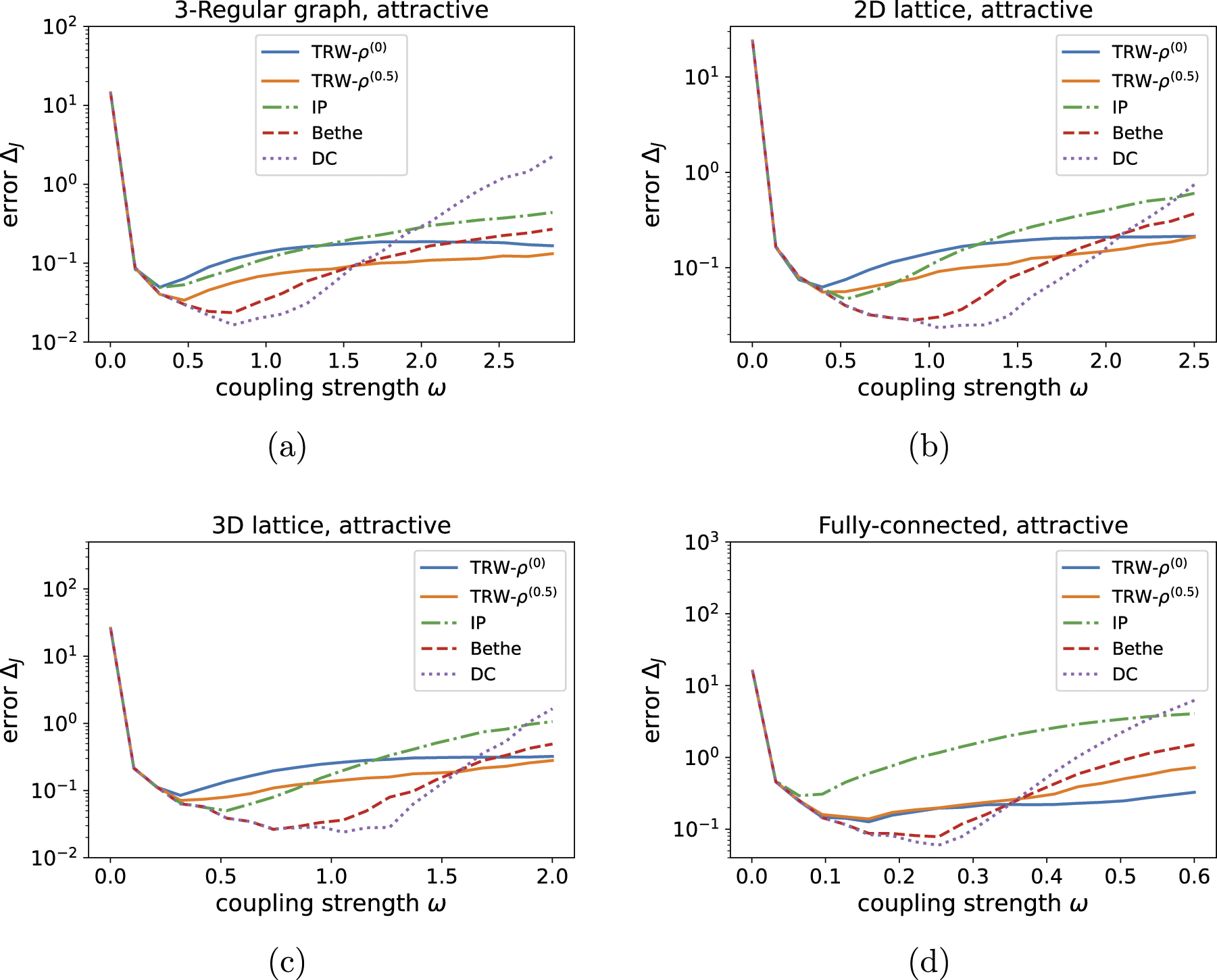
In figure 1, we show the reconstruction result for the attractive-interaction models. For all the graph structures and the inverse formulas, the error measurement Δ_J becomes large in the regions with small interaction strength ω. This is because in such small ω regions, the statistical uncertainty of the mean and covariance primarily dominates the errors, and the differences in the inverse formulas are completely eliminated [6, 19].

Zoom In Zoom Out Reset image size

When ω is nonzero, the differences between the inverse formulas become large. For all settings, the IP approximation typically gives the worst results. For the strongly attractive interactions, the proposed TRW approximation yields reasonable errors compared to the Bethe and DC inverse formulas. We next compare the uniform and weighted parameter settings of the TRW formulas, TRW-ρ⁽⁰⁾ and TRW-ρ^(0.5) respectively. For the sparse graphs, i.e. the regular and lattice graphs, TRW-ρ^(0.5) was better than TRW-ρ⁽⁰⁾, while TRW-ρ⁽⁰⁾ was better than TRW-ρ^(0.5) for the fully-connected graph. This is reasonable because for sparse graphs, a maximum spanning tree has a large responsibility in reconstruction of parameters, therefore giving a large weight to the maximum spanning tree may be helpful for the good reconstruction. On the other hand, for dense graphs, many spanning trees are important for the reconstruction, thus treating all the trees equally may make the reconstruction better. Especially, for large ω, TRW-ρ^(0.5) gave the best results for the regular and lattice graphs, and TRW-ρ⁽⁰⁾ gave the best for the fully-connected graph among all the inverse formula.

In figure 2, we show the reconstruction results for the mixed-interaction models. For the mixed interactions, the Bethe and DC approximations yield the best results for the lattice and fully-connected graphs in the region of large ω. For the three-regular graph, TRW-ρ^(0.5) and the Bethe formula were the best in the region of large ω. Comparing TRW-ρ⁽⁰⁾ and TRW-ρ^(0.5), we found the same tendency with the attractive case, i.e. TRW-ρ^(0.5) was better for the sparse graphs, but the superiority of TRW-ρ⁽⁰⁾ for the fully-connected graph was not clear and it showed almost the same accuracy with TRW-ρ^(0.5). Also for the fully-connected graph, the results of the both TRW approximations became comparable to those of the Bethe and DC approximations when the interactions are strong.

Zoom In Zoom Out Reset image size

Aiming at faster and more accurate learning, we developed a new, iteration-free formula for the inverse Ising problem. Following a previous study using the Bathe approximation [6], we combined the linear response relation and the pseudomoment-matching conditions to derive the inverse formula. However, we used the TRWfree energy rather than the Bethe free energy. The advantage of using the TRW free energy over the Bethe free energy is twofold. The first advantage is that the TRW free energy is convex, allowing us to find the global optimal solution. The second advantage is that we can optimize a rigorous lower bound on the likelihood function using the optimal value of the TRW free energy. We analytically obtained the TRW inverse formula (33), which gives the interaction matrix as a function of the edge appearance probabilities ρ_ij as well as the statistics of the input datasets m_i and C_ij . Using this formula, we could compute the approximate interaction matrix with the same computational complexity as in the Bethe approximation (35).

In order to use the TRW formula, we need to fix the edge appearance probability ρ_ij . We proposed two settings, ${\rho }_{ij}^{(0)}$ and ${\rho }_{ij}^{(0.5)}$. For ${\rho }_{ij}^{(0)}$, all edges are treated equivalently, while for ${\rho }_{ij}^{(0.5)}$, the edges in the maximum spanning tree are biased to have more weights. We called the TRW approximation with ${\rho }_{ij}^{(0)}$ and ${\rho }_{ij}^{(0.5)}$ as TRW-ρ⁽⁰⁾ and TRW-ρ^(0.5), respectively.

We compared the proposed TRW inverse formula to others in interaction reconstruction experiments in models with attractive and mixed interactions on various graph structures. We found that the TRW-ρ^(0.5) gave the best accuracy in models with large attractive interactions for the regular and lattice graphs, while the TRW-ρ⁽⁰⁾ was the best for the fully-connected graph. In particular, for the fully connected graph, the TRW-ρ⁽⁰⁾ formula showed overwhelmingly good reconstructions compared to the Bethe and DC approximations. In contrast, for mixed-interaction matrices (i.e. the elements were both positive and negative), the best estimations were typically obtained by the Bethe and DC approximations. However, the TRW-ρ^(0.5) formula gave the best results with large interactions on the regular graph.

We also found limitations to using the TRW inverse formula. The first limitation was the negative argument of the square root in the inverse formula (33): empirically, we found that when the interactions and biases were large, m_i also became large, and the argument tended to become negative, which resulted in the failure of the TRW approximation. Note that this limitation is also present in the Bethe inverse formula [6]. The second limitation was singular correlation matrices: if a correlation matrix was singular, we could not compute its inverse and could not use the TRW inverse formula. This situation was seen when the number of samples was too small or when the interaction was too large. The TRW, Bethe and DC inverse formulas all have this limitation. Interestingly, the IP inverse formula does not experience singular correlation matrices. The third limitation was that we needed the information of graph structure in advance to use the TRW inverse formula, because the graph structure is required in order to set ρ_ij . This limitation restricts the TRW formula from the applications such as estimation of a graph structure from data.

Although we demonstrated that the TRW inverse formula is useful, some open questions should be addressed for future improvements and practical applications. First, the TRW inverse formula has the free parameter ρ_ij , which was fixed to ${\rho }_{ij}^{(0)}$ and ${\rho }_{ij}^{(0.5)}$ in our experiments. There is no doubt that optimizing ρ_ij improves the accuracy of the inferred interactions. In fact, a method to obtain the optimal ρ_ij value that minimizes the upper bound Φ^TRW(J, h; ρ) has been previously discussed in the context of direct problems [11]. However, it is difficult to obtain an optimal value by analytically solving equations, and we must perform iterative computations. Even though it is difficult to analytically obtain the optimal value, there may be an easy but efficient choice of ρ_ij that is superior to the choices used in this study. It is also interesting to optimize the parameter α in ${\rho }_{ij}^{(\alpha )}$ in equation (44).

Another question is the extension of the inverse formula to models with hidden variables such as restricted Boltzmann machines. The introduction of hidden variables makes the model drastically simpler and recognizable to a human being. We may directly extend the inverse formula to include hidden variables, or we may use the inverse formula in a step of expectation-maximization-like algorithms to reduce the computational cost.

Finally, we are interested in applying TRW approximation and the proposed inverse formula to physics. The partition function dominates the physical properties of a system, such as phase transitions and critical phenomena. Thus, the TRW approximation, which can give a rigorous bound for the partition function, may be applicable to the mathematical analysis of physical models. The proposed formulation, with which we analyzed the exact solution of the TRW free energy, may also be useful for providing new insights into statistical and mathematical physics.

We are grateful to anonymous reviewers for helpful comments that significantly improved the paper. Part of this paper is based on results obtained from a project commissioned by the New Energy and Industrial Technology Development Organization (NEDO). This work was supported by JSPS KAKENHI Grant Nos. JP18K18117 and JP18K11488, and the INOUE ENRYO Memorial Grant, TOYO University. Some of the material in this paper has been reused from our preliminary conference paper, 'An Analytic Solution to the Inverse Ising Problem in the Tree-reweighted Approximation', in IEEE Proceedings, 2018, with permission, © 2022 IEEE.