Run-and-tumble motion in a harmonic potential: field theory and entropy production

Active matter encompasses reaction–diffusion systems out of equilibrium whose components are subject to local non-thermal forces [1]. There is a plethora of interesting patterns and phenomenology in this broad class of systems. Some fascinating examples are active nematics [2–4], active emulsions [5], and active motility [6, 7], among many others. Active matter has become a research focus in statistical mechanics over recent years, as it addresses fundamental questions on the physics of non-equilibrium systems, but also as a quantitative approach to biological physics and the path to designing an autonomous microbiological engine [8–11].

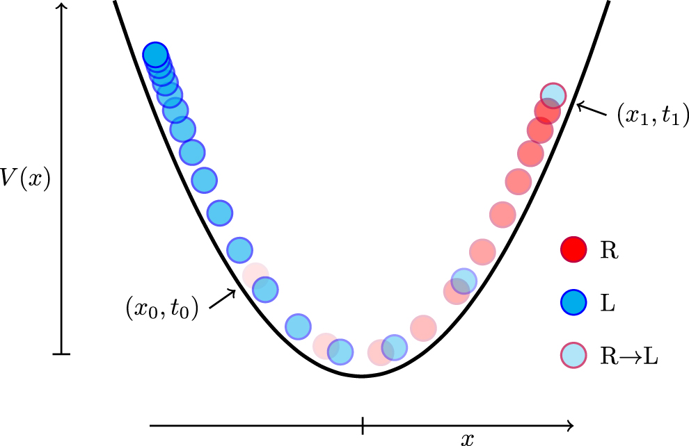
In this paper we study a model of active motility known as run and tumble (RnT) [12] that has been used to describe bacterial swimming patterns such as that of Escherichia coli and Salmonella [13]. A particle undergoing RnT motion moves in a sequence of runs at constant self-propulsion speed w interrupted by sudden changes (tumbles) in its orientation that happen at Poissonian rate α, [14–21]. This motion pattern is ballistic at the microscopic scale and diffusive at the large scale with effective diffusion constant D_eff = w²/α [12, 20, 22–27]. We study a RnT particle subject to thermal noise with diffusion constant D confined in a harmonic potential V(x) = kx²/2, see figure 1. The thermal noise is an important element in our derivation, as it allows the introduction of the Hermite orthogonal system, although it can later be switched off by taking the limit D → 0. Despite the stationary distribution has been derived in the limit D → 0 before [28], to our knowledge most of our results are novel for D > 0. Here we show how to derive a Doi-Peliti field theory for an RnT particle in a harmonic potential and calculate the short-time propagator; zeroth, first and second moments of the position of a right-moving particle; entropy production rate (or Kullback–Leibler distance between forward and backward paths); stationary distribution of the RnT particle and the right-moving particle; and other observables such as the mean-square displacement, the two-point correlation function, and the two-time correlation function. The stochastic process described above has a parallel in the context of gene regulation, where a gene switches back and forth between two states with different transcription rates. Gene transcription gives rise to a product (mRNA molecules) that is subject to decay (degradation of mRNA molecules) [29–32]. This biological process can be mapped to an RnT particle in a harmonic potential, where the gene state corresponds to the particle species (right- or left-moving), and the switching rates correspond to the tumbling rate α/2. The product concentration corresponds to the position of the particle x, the transcription rates correspond to the self-propulsion speeds, and the degradation rate corresponds to the potential strength k. This model is closer to the biological process if we allow for asymmetric transcription and switching rates, which correspond to asymmetric self-propulsion speeds and tumbling rates. We discuss this generalisation of RnT motion in appendix A.

In this paper, we follow a path integral approach [15] whereby we derive a perturbative field theory in the Doi-Peliti framework [33] and use it to calculate a number of observables in closed form, with an emphasis on the entropy production [34]. Despite our approach being perturbative, all our results are exact. The presence of the external potential presents technical challenges in the derivation of the field theory that resemble those encountered in other contexts such as the quantum harmonic oscillator [35–37]. We use a combination of the Fourier transform and Hermite polynomials to parametrise the fields as to diagonalise the action functional.

We regard the Doi-Peliti framework as a method to solve a master equation, or a Fokker–Planck equation of a particle system. It therefore crucially retains the microscopic dynamics of the system and captures the particle nature of the constituent degrees of freedom, see appendix H. For this reason, the Doi-Peliti framework provides a solid route to calculate the entropy production and, most importantly, proves itself to be an effective tool to study active particle systems. In this paper, we illustrate this point by studying RnT motion. We regard the present work as the foundation to address a number of important questions about interacting active matter, such as the microscopics of motility induced phase separation, an active kinetic theory and how to extract useful work from active matter.

The contents of this paper are organised as follows: in section 2, we derive a field theory for an RnT particle in a harmonic potential; in section 3 we use this field theory to calculate the entropy production; and in section 4 we discuss our results. In the appendix, we have included other relevant observables: mean square displacement (appendix F), two-point correlation functions (appendices H and I), expected velocity (appendix G), and stationary distribution (appendix D).

Zoom In Zoom Out Reset image size

In one dimension, we can think of RnT motion as the interaction between right- and left-moving particles that transmute into one another at Poissonian rate α/2, see figure 1. The Langevin equations of each species are

$$\begin{equation}{\dot {x}}_{\phi }=-{\partial }_{x}V\left(x\right)+w+\eta \left(t\right)\end{equation} \tag{ 1 }$$

for right-moving particles and

$$\begin{equation}{\dot {x}}_{\psi }=-{\partial }_{x}V\left(x\right)-w+\eta \left(t\right)\end{equation} \tag{ 2 }$$

for left-moving particles, where η is a Gaussian white noise with mean $\left\langle \eta \left(t\right)\right\rangle =0$ and correlation function $\left\langle \eta \left(t\right)\eta \left({t}^{\prime }\right)\right\rangle =2D\delta \left(t-{t}^{\prime }\right)$, with diffusion constant D. The corresponding Fokker–Planck equations are coupled due to the transmutation between species through a gain and loss terms,

$$\begin{equation}{\partial }_{t}{P}_{\phi }=-{\partial }_{x}\left[\left(-kx+w\right){P}_{\phi }\right]+D{\partial }_{x}^{2}{P}_{\phi }+\frac{\alpha }{2}\left({P}_{\psi }-{P}_{\phi }\right),\end{equation} \tag{ 3a }$$

$$\begin{equation}{\partial }_{t}{P}_{\psi }=-{\partial }_{x}\left[\left(-kx-w\right){P}_{\psi }\right]+D{\partial }_{x}^{2}{P}_{\psi }+\frac{\alpha }{2}\left({P}_{\phi }-{P}_{\psi }\right),\end{equation} \tag{ 3b }$$

where P_ϕ (x, t) and P_ψ (x, t) are the probability densities of a right- and a left-moving particle respectively, as a function of position x and time t. As we show throughout this paper, the symmetry between right- and left-moving particles due to isotropic self-propulsion velocities and equal tumbling rates turns out to simplify our derivations. However, our results can be generalised to the asymmetric case, with anisotropic self-propulsion and different tumbling rates, which we discuss in appendix A.

Most of the results that follow can be derived directly from the Langevin equations (1) and (2), and Fokker–Planck equation (3) via classic probabilistic methods. However, we follow instead a Doi-Peliti path integral approach because it provides a systematic route to calculate results using perturbative expansions. Moreover, in this framework, the stochastic system can be easily extended to include other interactions and particle species, and allows for tools such as renormalisation Group that are not available in classic methods. These features are essential for our current and future research in active matter.

In the following we show how to derive a Doi-Peliti field theory of our system. Without having to translate the Langevin equations in (1) and (2) to the lattice and later taking the continuum limit, we write the action functional straightaway from the Fokker–Planck equation (3) as shown in [38],

$$\begin{align}\mathcal{A}& =\int \mathrm{d}x\enspace \enspace \mathrm{d}t\enspace \left\{\tilde {\phi }\left({\partial }_{t}\phi +{\partial }_{x}\left[\left(-kx+w\right)\phi \right]-D{\partial }_{x}^{2}\phi \right)\right.\\ & \quad \left.+\tilde {\psi }\left({\partial }_{t}\psi +{\partial }_{x}\left[\left(-kx-w\right)\psi \right]-D{\partial }_{x}^{2}\psi \right)+\frac{\alpha }{2}\left(\tilde {\phi }-\tilde {\psi }\right)\left(\phi -\psi \right)\right\},\end{align} \tag{ 4 }$$

where ϕ is the annihilation field of right-moving particles; $\tilde {\phi }$ is the Doi-shifted [39] creation field ${\phi }^{{\dagger}}=\tilde {\phi }+1$ of right-moving particles; ψ is the annihilation field of left-moving particles; and $\tilde {\psi }$ is the Doi-shifted creation field ${\psi }^{{\dagger}}=\tilde {\psi }+1$ of left-moving particles. The action functional (4) allows the calculation of an observable • via the path integral

$$\begin{equation}\left\langle {\bullet}\right\rangle =\int \mathcal{D}\left[\phi ,\tilde {\phi },\psi ,\tilde {\psi }\right]{\bullet}{e}^{-\mathcal{A}\left(\left[\phi ,\tilde {\phi },\psi ,\tilde {\psi }\right]\right)}.\end{equation} \tag{ 5 }$$

The action in equation (4) contains only bilinear terms, where the only interaction between species is due to transmutation. This action does not have any non-linear couplings. Motivated by the matrix representation of the action (4), we refer to any terms involving $\tilde {\phi }\phi$ or $\tilde {\psi }\psi$ as diagonal terms, and to the terms $\tilde {\phi }\psi$ and $\tilde {\psi }\phi$ as off-diagonal terms. The diagonal terms in (4) are semi-local due to the derivatives in space and time, which need to be made local in order to carry out the Gaussian (path) integral. This is usually achieved by expressing the fields in Fourier space. In this case, however, Fourier-transforming (4) yields the action local in the frequency ω but not in position x Fourier-transformed. Due to the diagonal terms $-k\tilde {\phi }{\partial }_{x}\left(x\phi \right)\enspace -k\tilde {\psi }{\partial }_{x}\left(x\psi \right)$, the action remains semi-local after Fourier-transforming.

Instead, we first parametrise the action by the density field $\rho =\left(\phi +\psi \right)/\sqrt{2}$ and the polarity field $\nu =\left(\phi -\psi \right)/\sqrt{2}$, also called chirality [40], with the analogous transformation for the conjugate fields. This change of variables is useful in other contexts and is known under other names, such as the Keldysh rotation [41]. In our case, the advantage is that the action remains invariant under the transformation ρ ↔ ν, $\tilde {\rho }{\leftrightarrow}\tilde {\nu }$, except for the mass term $\alpha \tilde {\nu }\nu$,

$$\begin{align}\mathcal{A}& =\int \mathrm{d}x\enspace \enspace \mathrm{d}\hspace{-1.5pt}\bar\;\omega \enspace \{-\mathring{{\imath}}\omega \tilde {\rho }\rho -k\tilde {\rho }{\partial }_{x}(x\rho )-D\tilde {\rho }{\partial }_{x}^{2}\rho -\mathring{{\imath}}\omega \tilde {\nu }\nu -k\tilde {\nu }{\partial }_{x}(x\nu )\\ & \quad -D\tilde {\nu }{\partial }_{x}^{2}\nu +\alpha \tilde {\nu }\nu +w\tilde {\rho }{\partial }_{x}\nu +w\tilde {\nu }{\partial }_{x}\rho \}.\end{align} \tag{ 6 }$$

We then use the solution to the eigenvalue problem $\mathcal{L}\left[u\left(x\right)\right]=\lambda u\left(x\right)$, with

$$\begin{equation}\mathcal{L}\left[u\left(x\right)\right]={\partial }_{x}^{2}u\left(x\right)+{\partial }_{x}\left(x\enspace u\left(x\right)\right)/{L}^{2},\end{equation} \tag{ 7 }$$

$L=\sqrt{D/k}$ and $\lambda \in \mathbb{R}$, where the differential operator follows from the diagonal terms in (6). By using the fields ρ and ν, instead of the original ϕ and ψ, we have the same differential operator $\mathcal{L}$ acting on both ρ and ν.

The solution to this eigenvalue problem is the set of functions

$$\begin{equation}{u}_{n}\left(x\right)={e}^{-\frac{{x}^{2}}{2{L}^{2}}}\enspace {H}_{n}\left(\frac{x}{L}\right),\end{equation} \tag{ 8 }$$

with eigenvalue λ_n = −n/L², where ${H}_{n}\left(x\right)$ is the nth Hermite polynomial in the 'probabilists' convention', see appendix B [35, 42–44]. The functions u_n (x) are similar to the so-called Hermite functions $\mathrm{exp} \left(-{x}^{2}/\left(4{L}^{2}\right)\right)\enspace {H}_{n}\left(x/L\right)$. Defining the set of functions

$$\begin{equation}{\tilde {u}}_{n}\left(x\right)=\frac{1}{\sqrt{2\pi }\enspace n!}{H}_{n}\left(\frac{x}{L}\right),\end{equation} \tag{ 9 }$$

the orthogonality relation between u_n (x) and ${\tilde {u}}_{m}\left(x\right)$ follows from the orthogonality of Hermite polynomials in equation (B.2),

$$\begin{equation}{\int }_{-\infty }^{\infty } \mathrm{d}x\enspace \enspace {u}_{n}\left(x\right){\tilde {u}}_{m}\left(x\right)=L\enspace {\delta }_{n,m},\end{equation} \tag{ 10 }$$

where δ_n,m is the Kronecker δ. We can now use u_n and ${\tilde {u}}_{m}$ as basis for the fields ρ, $\tilde {\rho }$, ν and $\tilde {\nu }$,

$$\begin{equation}\left(\sim \right){\rho }\left(x,t\right)=\int \mathrm{d}\hspace{-1.5pt}\bar\;\omega \enspace \enspace {e}^{-\mathring{{\imath}}\omega t}\frac{1}{L}\sum\limits _{n}{\left(\sim \right){\rho }}_{n}\left(\omega \right){\left(\sim \right){u}}_{n}\left(x\right),\end{equation} \tag{ 11a }$$

$$\begin{equation}\left(\sim \right){\nu }\left(x,t\right)=\int \mathrm{d}\hspace{-1.5pt}\bar\;\omega \enspace \enspace {e}^{-\mathring{{\imath}}\omega t}\frac{1}{L}\sum\limits _{n}{\left(\sim \right){\nu }}_{n}\left(\omega \right){\left(\sim \right){u}}_{n}\left(x\right).\end{equation} \tag{ 11b }$$

Using the representation (11) and the orthogonality relation (10) in the action $\mathcal{A}={\mathcal{A}}_{0}+{\mathcal{A}}_{1}$ in (6), we have

$$\begin{align}{\mathcal{A}}_{0}& =\frac{1}{{L}^{2}}\sum\limits _{n,m}L{\delta }_{n,m}\int \mathrm{d}\hspace{-1.5pt}\bar\;\omega \enspace \enspace \mathrm{d}\hspace{-1.5pt}\bar{\;\omega }^{\prime }\enspace \delta \hspace{-2.5pt}\bar\;\left(\omega +{\omega }^{\prime }\right)\\ & \quad {\times}\left[\left(-\mathring{{\imath}}\omega +kn\right){\tilde {\rho }}_{n}\left({\omega }^{\prime }\right){\rho }_{m}\left(\omega \right)+\left(-\mathring{{\imath}}\omega +kn+\alpha \right){\tilde {\nu }}_{n}\left({\omega }^{\prime }\right){\nu }_{m}\left(\omega \right)\right],\end{align} \tag{ 12a }$$

$$\begin{equation}{\mathcal{A}}_{1}=-\frac{w}{L}\frac{1}{{L}^{2}}\sum\limits _{n,m}L{\delta }_{n-1,m}\int \mathrm{d}\hspace{-1.5pt}\bar\;\omega \enspace \enspace \mathrm{d}\hspace{-1.5pt}\bar{\;\omega }^{\prime }\enspace \delta \hspace{-2.5pt}\bar\;\left(\omega +{\omega }^{\prime }\right)\left[{\tilde {\rho }}_{n}\left({\omega }^{\prime }\right){\nu }_{m}\left(\omega \right)+{\tilde {\nu }}_{n}\left({\omega }^{\prime }\right){\rho }_{m}\left(\omega \right)\right],\end{equation} \tag{ 12b }$$

where ${\mathcal{A}}_{0}$ contains the local, diagonal terms and ${\mathcal{A}}_{1}$ contains the off-diagonal terms, which are non-local due to δ_n−1,m . We can then regard ${\mathcal{A}}_{0}$ as the Gaussian model and ${\mathcal{A}}_{1}$ as a perturbation about it.

The Gaussian model corresponds to Ornstein–Uhlenbeck particles where one species has decay rate α. Defining an observable • in the Gaussian model as

$$\begin{equation}{\left\langle {\bullet}\right\rangle }_{0}=\int \mathcal{D}\left[\rho ,\tilde {\rho },\nu ,\tilde {\nu }\right]{\bullet}\enspace {e}^{-{\mathcal{A}}_{0}\left(\left[\rho ,\tilde {\rho },\nu ,\tilde {\nu }\right]\right)},\end{equation} \tag{ 13 }$$

from (5) it follows that the perturbation expansion of the observable in the full model, the RnT particle, is

$$\begin{equation}\left\langle {\bullet}\right\rangle ={\left\langle {\bullet}\enspace {e}^{-{\mathcal{A}}_{1}}\right\rangle }_{0}=\sum\limits _{N=0}^{\infty }\frac{1}{N!}{\left\langle {\bullet}{\left(-{\mathcal{A}}_{1}\right)}^{N}\right\rangle }_{0}.\end{equation} \tag{ 14 }$$

By performing the Gaussian path integral [45] in (13), the bare propagators read

where r is a mass term added to regularise the infrared divergence and which is to be taken to 0 when calculating any observable. We use Feynman diagrams to represent propagators [33, 39, 45], where time (causality) is read from right to left. On the other hand, we have

$$\begin{equation}{\langle {\rho }_{n}\left(\omega \right){\tilde {\nu }}_{m}\left({\omega }^{\prime }\right)\rangle }_{0}=\enspace 0,\end{equation} \tag{ 16a }$$

$$\begin{equation}{\langle {\nu }_{n}\left(\omega \right){\tilde {\rho }}_{m}\left({\omega }^{\prime }\right)\rangle }_{0}=\enspace 0,\end{equation} \tag{ 16b }$$

for any n, m, which implies that there is no 'interaction' between ρ and ν at the bare level. The perturbative part ${\mathcal{A}}_{1}$ of the action, equation (12b), however, provides the amputated vertices

which shift the index by one. As the coupling $w/L=w\sqrt{k/D}$ diverges for small D, more and more perturbative terms have to be taken into account in the limit of small D, figure D1.

2.1. Full propagator in reciprocal space

To calculate certain observables such as the time-dependent probability distribution of the RnT particle, we need the full propagators. To derive the full propagators we use the action in (12), the bare propagators in (15), (16), the perturbative vertex (17), as well as Wick's Theorem [45]. Consider, for instance, the propagator of the density field $\left\langle \rho \tilde {\rho }\right\rangle$. From (14) we have

where the zeroth order term is given in equation (15a) and the first order term is

$$\begin{equation}{\left\langle {\rho }_{n}\left(\omega \right){\tilde {\rho }}_{m}\left({\omega }^{\prime }\right)\left(-{\mathcal{A}}_{1}\right)\right\rangle }_{0}=\enspace 0.\end{equation} \tag{ 19 }$$

Equation (18) allows us to calculate the stationary distribution, appendix D. The second order term in (18) is

using two of the index-shifting vertices (17). From (16a) it follows that any term in (18) of odd order N vanishes because the fields ρ, $\tilde {\rho }$, ν and $\tilde {\nu }$ cannot be paired according to (15). Then, the contributions to the full propagator $\left\langle \rho \tilde {\rho }\right\rangle$ are

$$\begin{align}& \frac{1}{N!}{\left\langle {\rho }_{n}\left(\omega \right){\tilde {\rho }}_{m}\left({\omega }^{\prime }\right){\left(-{\mathcal{A}}_{1}\right)}^{N}\right\rangle }_{0}\\ & \hspace{25.0pt}=\begin{cases}L{\delta }_{n,m+N}\delta \hspace{-2.5pt}\bar\;\left(\omega +{\omega }^{\prime }\right){\left(\frac{w}{L}\right)}^{N}\prod\limits _{j=0}^{N}\frac{1}{-\mathring{{\imath}}\omega +k\left(m+j\right)+{p}_{j}}\quad & \quad \text{if}\enspace N\;\text{even},\\ 0\quad & \quad \text{if}\enspace N\;\text{odd},\end{cases}\end{align} \tag{ 21 }$$

where p_j = r if j is even and p_j = α if j is odd. Similarly, the contributions to the full propagators $\left\langle \nu \tilde {\nu }\right\rangle$, $\left\langle \rho \tilde {\nu }\right\rangle$ and $\left\langle \nu \tilde {\rho }\right\rangle$ are, respectively,

$$\begin{align}& \frac{1}{N!}{\left\langle {\nu }_{n}\left(\omega \right){\tilde {\nu }}_{m}\left({\omega }^{\prime }\right){\left(-{\mathcal{A}}_{1}\right)}^{N}\right\rangle }_{0}\\ & \hspace{25.0pt}=\begin{cases}L{\delta }_{n,m+N}\delta \hspace{-2.5pt}\bar\;\left(\omega +{\omega }^{\prime }\right){\left(\frac{w}{L}\right)}^{N}\prod\limits _{j=0}^{N}\frac{1}{-\mathring{{\imath}}\omega +k\left(m+j\right)+{q}_{j}}\quad & \quad \text{if}\enspace N\;\text{even},\\ 0\quad & \quad \text{if}\enspace N\;\text{odd},\end{cases}\end{align} \tag{ 22a }$$

$$\begin{align}& \frac{1}{N!}{\left\langle {\rho }_{n}\left(\omega \right){\tilde {\nu }}_{m}\left({\omega }^{\prime }\right){\left(-{\mathcal{A}}_{1}\right)}^{N}\right\rangle }_{0}\\ & \hspace{25.0pt}=\begin{cases}0\quad & \quad \text{if}\enspace N\;\text{even},\\ L{\delta }_{n,m+N}\delta \hspace{-2.5pt}\bar\;\left(\omega +{\omega }^{\prime }\right){\left(\frac{w}{L}\right)}^{N}\prod\limits _{j=0}^{N}\frac{1}{-\mathring{{\imath}}\omega +k\left(m+j\right)+{q}_{j}}\quad & \quad \text{if}\enspace N\;\text{odd},\end{cases}\end{align} \tag{ 22b }$$

$$\begin{align}& \frac{1}{N!}{\left\langle {\nu }_{n}\left(\omega \right){\tilde {\rho }}_{m}\left({\omega }^{\prime }\right){\left(-{\mathcal{A}}_{1}\right)}^{N}\right\rangle }_{0}\\ & \hspace{25.0pt}=\begin{cases}0\quad & \quad \text{if}\enspace N\;\text{even},\\ L{\delta }_{n,m+N}\delta \hspace{-2.5pt}\bar\;\left(\omega +{\omega }^{\prime }\right){\left(\frac{w}{L}\right)}^{N}\prod\limits _{j=0}^{N}\frac{1}{-\mathring{{\imath}}\omega +k\left(m+j\right)+{p}_{j}}\quad & \quad \text{if}\enspace N\;\text{odd},\end{cases}\end{align} \tag{ 22c }$$

where q_j = α if j is even and q_j = r if j is odd. The diagrammatic representation of the full propagators is

where the black circle • represents the sum over all possible diagrams that have the same incoming and outgoing legs. Some of these propagators are calculated in closed form in appendix C.

2.2. Short-time propagator in real space

In this section we calculate the short-time propagator ${\langle \phi \left(y,\tau \right)\tilde {\phi }\left(x,0\right)\rangle }_{1}$ of a right-moving particle that moves from position x to y in an interval of time τ, and the short-time propagator ${\langle \psi \left(y,\tau \right)\tilde {\phi }\left(x,0\right)\rangle }_{1}$ of a right-moving particle x that transmutates into a left-moving particle at y in an interval of time τ. The subindex indicates that the propagator is expanded to first order about the Gaussian model, ${\langle {\bullet}\rangle }_{1}={\langle {\bullet}\rangle }_{0}-{\langle {\bullet}{\mathcal{A}}_{1}\rangle }_{0}$. Expanding to Nth order in the perturbative part of the action generally provides the Nth order in τ [38]. Using the recurrence relation (B.6), Mehler's formula (B.7) and the propagators in equations (C.1)–(C.6), these two propagators are,

$$\begin{align}& \hspace{25.0pt}=\frac{1}{2}\sqrt{\frac{k}{2\pi D\left(1-\mathrm{exp} \left(-2k\tau \right)\right)}}\enspace {e}^{-\frac{k{\left(y-x\enspace \mathrm{exp}\left(-k\tau \right)\right)}^{2}}{2D\left(1-\mathrm{exp}\left(-2k\tau \right)\right)}}\\ & \quad \hspace{25.0pt}{\times}\left(1+{e}^{-\alpha \tau }+\frac{wk\left(y-x{e}^{-k\tau }\right)}{D\left(1-{e}^{-2k\tau }\right)}\left[\frac{1}{k-\alpha }\left(\enspace {e}^{-\alpha \tau }-{e}^{-k\tau }\right)\right.\right.\\ & \hspace{25.0pt}\quad +\left.\left.\frac{1}{k+\alpha }\left(1-{e}^{-\left(k+\alpha \right)\tau }\right)\right]\right)\end{align} \tag{ 24b }$$

$$\begin{align}& \hspace{25.0pt}=\frac{1}{\sqrt{4\pi D\tau }}\enspace {e}^{-\frac{{\left(y-x\left(1-k\tau \right)\right)}^{2}}{4D\tau }}\left(1+\frac{w\left(y-x\right)}{2D}\right.\\ & \quad \hspace{25.0pt}+\left.\left(-\frac{\alpha }{2}+\frac{w}{4D}\left(k\left(y+x\right)-\alpha \left(y-x\right)\right)\right)\tau +\mathcal{O}\left({\tau }^{2}\right)\right),\end{align} \tag{ 24c }$$

and

$$\begin{align}& \hspace{25.0pt}=\frac{1}{2}\sqrt{\frac{k}{2\pi D\left(1-\mathrm{exp} \left(-2k\tau \right)\right)}}\enspace {e}^{-\frac{k{\left(y-x\enspace \mathrm{exp}\left(-k\tau \right)\right)}^{2}}{2D\left(1-\mathrm{exp}\left(-2k\tau \right)\right)}}\\ & \hspace{25.0pt}\quad {\times}\left(1-{e}^{-\alpha \tau }+\frac{wk\left(y-x{e}^{-k\tau }\right)}{D\left(1-{e}^{-2k\tau }\right)}\left[\frac{1}{k-\alpha }\left(\enspace {e}^{-\alpha \tau }-{e}^{-k\tau }\right)\right.\right.\\ & \quad \hspace{25.0pt}-\left.\left.\frac{1}{k+\alpha }\left(1-{e}^{-\left(k+\alpha \right)\tau }\right)\right]\right)\end{align} \tag{ 25b }$$

$$\begin{equation}\hspace{25.0pt}=\frac{1}{\sqrt{4\pi D\tau }}\enspace {e}^{-\frac{{\left(y-x\left(1-k\tau \right)\right)}^{2}}{4D\tau }}\left(\frac{\alpha }{2}\tau +\mathcal{O}\left({\tau }^{2}\right)\right).\end{equation} \tag{ 25c }$$

Comparing (24) with (25) we see that the transition probability that involves exactly one transmutation event, independently of displacement, is of higher order in τ than the transition probability of just a displacement.

2.3. Zeroth, first and second moments of the position of a right-moving particle

As it will become clear in section 3, we need the zeroth, first and second moments of the position of a right-moving particle to calculate the entropy production of an RnT particle in a harmonic potential. Assuming that the system is initialised with a right-moving particle placed at x₀ at time t₀ = 0, the nth moment of its position is

$$\begin{equation}\left\langle {x}_{\phi }^{n}\left(t\right)\right\rangle ={\int }_{-\infty }^{\infty } \mathrm{d}x\enspace \enspace {x}^{n}\langle \phi \left(x,t\right)\tilde {\phi }\left({x}_{0},0\right)\rangle ,\end{equation} \tag{ 26 }$$

where the propagator $\langle \phi \left(x,t\right)\tilde {\phi }\left({x}_{0},0\right)\rangle$ expressed in terms of the $\left(\sim \right){\rho }$ and $\left(\sim \right){\nu }$ fields contains the four full propagators, , equation (23). Definition (26) contains a mild abuse of notation that we will keep committing throughout, as the angular brackets were introduced in (5) as a path integral but are expectation over a density in (26). Since there is an integral over space and xⁿ is a polynomial in x, the observable can be written as linear combinations of Hermite polynomials, which simplifies the calculations by virtue of the orthogonality relation in (B.2). In particular, for the first three moments, $1={H}_{0}\left(x/L\right)$, $x/L={H}_{1}\left(x/L\right)$ and ${\left(x/L\right)}^{2}={H}_{0}\left(x/L\right)+{H}_{2}\left(x/L\right)$. Using the representation in (11) and the propagators derived in appendix C, the zeroth, first (see figure 2) and second moments are

From the propagators in equations (C.1)–(C.6), we see that at stationarity, only those terms remain where the Doi-shifted creation field is ${\tilde {\rho }}_{0}$. Then, equation (27) simplify to

$$\begin{equation}\underset{t\to \infty }{\mathrm{lim}}\enspace \left\langle {x}_{\phi }^{0}\left(t\right)\right\rangle =\frac{1}{2}\end{equation} \tag{ 28a }$$

$$\begin{equation}\underset{t\to \infty }{\mathrm{lim}}\enspace \left\langle {x}_{\phi }^{1}\left(t\right)\right\rangle =\frac{1}{2}\frac{w}{k+\alpha }\end{equation} \tag{ 28b }$$

$$\begin{equation}\underset{t\to \infty }{\mathrm{lim}}\enspace \left\langle {x}_{\phi }^{2}\left(t\right)\right\rangle =\frac{D}{2k}+\frac{{w}^{2}}{2k\left(k+\alpha \right)}\end{equation} \tag{ 28c }$$

at stationarity.

Zoom In Zoom Out Reset image size

In this section we derive the internal entropy production rate ${\dot {S}}_{i}$ at stationarity [46–49], assuming that the observer is able to distinguish whether the RnT particle is in its right- or left-moving state. We discuss the case where the observer is not able to distinguish the RnT particle's state in appendix E. Other observables we calculate are in the appendix: mean square displacement (appendix F), two-point correlation function (appendix H), two-time correlation function (appendix I), expected velocity (appendix G) and stationary distribution (appendix D).

The internal entropy production is defined as the Kullback–Leibler distance between forward and backward paths [38, 46, 50]. Because the particle's position and species are Markov, the entropy production can easily be expanded in terms of the short-time propagators [51]

$$\begin{align}{\dot {S}}_{i}\left(t\right)& =\underset{\tau \to 0}{\mathrm{lim}}\frac{1}{2\tau }\int \mathrm{d}x\enspace \enspace \mathrm{d}y\enspace \left[P\left(x,t\right)W\left(x\to y;\tau \right)-P\left(y,t\right)W\left(y\to x;\tau \right)\right]\\ & \quad {\times}\mathrm{ln}\left(\frac{P\left(x,t\right)W\left(x\to y;\tau \right)}{P\left(y,t\right)W\left(y\to x;\tau \right)}\right),\end{align} \tag{ 29 }$$

where P(x, t) is the probability that the system is in state x at time t and W(x → y; τ) is the transition probability of the system to change from state x to y in an interval of time τ. The internal entropy production rate ${\dot {S}}_{i}$ is non-negative, and it is zero if and only if detailed balance P(x, t)W(x → y; τ) = P(y, t)W(y → x; τ) is satisfied for any two pairs of states x and y. A positive entropy production rate is thus the signature of non-equilibrium and it indicates the breakdown of time-reversal symmetry. The entropy production ${\dot {S}}_{i}\left(t\right)$ of a drift-diffusive particle in free space with velocity w and diffusion constant D is known to be ${\dot {S}}_{i}\left(t\right)=1/\left(2t\right)+{w}^{2}/D$ [46], where the first contribution is due to the relaxation to steady state and is independent of the system parameters, and the second contribution is due to the steady-state probability current.

We can anticipate that the stationary entropy production rate ${\dot {S}}_{i}$ of an RnT particle in a harmonic potential is positive given that, between tumbles, the particle is drift-diffusive and, therefore, there is locally a perpetual current. Moreover, a particle's forward trajectory, such as in figure 1, is distinct from its backwards trajectory, which indicates the breakdown of time-reversal symmetry.

Given the RnT particle is confined in a potential, its probability distribution develops into a stationary state, see appendix D. We denote the stationary distribution by P(x) = lim_t→∞  P(x, t). In the following, we derive the stationary ${\dot {S}}_{i}={\mathrm{lim}}_{t\to \infty }\enspace {\dot {S}}_{i}\left(t\right)$ in (29) along the lines of [46, 51].

First, the contribution of P(x) in the logarithm vanishes at stationarity,

$$\begin{equation}\int \mathrm{d}x\enspace \enspace \mathrm{d}y\enspace \left[P\left(x\right)W\left(x\to y;\tau \right)-P\left(y\right)W\left(y\to x;\tau \right)\right]\mathrm{ln}\left(\frac{P\left(x\right)}{P\left(y\right)}\right)=0,\end{equation} \tag{ 30 }$$

because of (i) the Markovian property, ∫dyW(x → y; τ) = 1, which implies ∫dyP(x)W(x → y; τ) = P(x), and (ii) the identity for Markov processes at stationarity, ∫dxP(x)W(x → y; τ) = P(y). Using (30) in (29) yields

$$\begin{equation}{\dot {S}}_{i}=\underset{\tau \to 0}{\mathrm{lim}}\enspace \frac{1}{2\tau }\int \mathrm{d}x\enspace \enspace \mathrm{d}y\enspace \left[P\left(x\right)W\left(x\to y;\tau \right)-P\left(y\right)W\left(y\to x;\tau \right)\right]\mathrm{ln}\left(\frac{W\left(x\to y;\tau \right)}{W\left(y\to x;\tau \right)}\right).\end{equation} \tag{ 31 }$$

Second, using the convention W(y → x; 0) = δ(x − y), we have

$$\begin{equation}-P\left(x\right)W\left(x\to y;0\right)+P\left(y\right)W\left(y\to x;0\right)=0,\end{equation} \tag{ 32 }$$

which we introduce in the square brackets in (31), to write ${\mathrm{lim}}_{\tau \to 0}\left(W\left(y\to x;\tau \right)-W\left(y\to x;0\right)\right)/\tau ={\mathrm{lim}}_{\tau \to 0}\enspace \dot {W}\left(x\to y;\tau \right)$, so that

$$\begin{equation}{\dot {S}}_{i}=\underset{\tau \to 0}{\mathrm{lim}}\enspace \frac{1}{2}\int \mathrm{d}x\enspace \enspace \mathrm{d}y\enspace \left[P\left(x\right)\dot {W}\left(x\to y;\tau \right)-P\left(y\right)\dot {W}\left(y\to x;\tau \right)\right]\mathrm{ln}\left(\frac{W\left(x\to y;\tau \right)}{W\left(y\to x;\tau \right)}\right),\end{equation} \tag{ 33 }$$

And third, expanding the square bracket in (33) and changing x ↔ y in one of the integrals gives

$$\begin{equation}{\dot {S}}_{i}=\underset{\tau \to 0}{\mathrm{lim}}\int \mathrm{d}x\enspace \enspace \mathrm{d}y\enspace P\left(x\right)\dot {W}\left(x\to y;\tau \right)\mathrm{ln}\left(\frac{W\left(x\to y;\tau \right)}{W\left(y\to x;\tau \right)}\right).\end{equation} \tag{ 34 }$$

Since the entropy production involves the limit τ → 0 of the transition rate $\dot {W}=\frac{\mathrm{d}}{\mathrm{d}\tau }W$, the entropy production crucially draws on the microscopic dynamics of the process. We can therefore focus on lower order contributions to $\dot {W}$ in τ and neglect higher order contributions.

For an RnT particle, all possible transitions between states involve a displacement (run) and/or a change in the direction of the drift (tumble). Given that, at stationarity, there is a symmetry between right- and left-moving particles under the transformation x ↔ −x, we can summarise the contributions to the entropy production (34) as

$$\begin{align}{\dot {S}}_{i}& =\underset{\tau \to 0}{\mathrm{lim}}\;2\int \mathrm{d}x\enspace \enspace \mathrm{d}y\enspace \enspace {P}_{\phi }\left(x\right)\left[\dot {W}\left(x\to y,\phi ;\tau \right)\mathrm{ln}\left(\frac{W\left(x\to y,\phi ;\tau \right)}{W\left(y\to x,\phi ;\tau \right)}\right)\right.\\ & \quad \left.+\dot {W}\left(x\to y,\phi \to \psi ;\tau \right)\mathrm{ln}\left(\frac{W\left(x\to y,\phi \to \psi ;\tau \right)}{W\left(y\to x,\psi \to \phi ;\tau \right)}\right)\right],\end{align} \tag{ 35 }$$

where ${P}_{\phi }\left(x\right)={\mathrm{lim}}_{t\to \infty }\enspace \langle \phi \left(x,t\right)\tilde {\phi }\left({x}_{0},0\right)\rangle$, which normalises to 1/2. The first term in the square bracket in (35) corresponds to the displacement of a right-moving particle from x to y with transition probability $W\left(x\to y,\phi ;\tau \right)=\langle \phi \left(y,\tau \right)\tilde {\phi }\left(x,0\right)\rangle$. The second term in the square bracket of (35) corresponds to the displacement of a particle from x to y that starts as right-moving and ends as left-moving, with transition probability $W\left(x\to y,\phi \to \psi ;\tau \right)=\langle \psi \left(y,\tau \right)\tilde {\phi }\left(x,0\right)\rangle$. These two transitions include any intermediate state where there may be displacement and transmutation, although their transition probabilities are of higher order in τ and therefore can be neglected. We therefore use the short-time propagators in (24) and (25) [38, 46].

In the following, we analyse which terms in (35) contribute to the entropy production rate ${\dot {S}}_{i}$. We first consider the transition due to transmutation and displacement, whose short-time propagator is (25). By symmetry, we see that the transition probability corresponding to displacement and transmutation in the short-time limit is

$$\begin{equation}W\left(x\to y,\phi \to \psi ;\tau \right)=W\left(-x\to -y,\psi \to \phi ;\tau \right)=\frac{1}{\sqrt{4\pi D\tau }}\enspace {e}^{-\frac{{\left(y-x\right)}^{2}}{4D\tau }}\left(\frac{\alpha }{2}\tau +\mathcal{O}\left({\tau }^{2}\right)\right),\end{equation} \tag{ 36 }$$

which is equal for the forward and backward trajectories. As the logarithm vanishes, the second term in (35) does not contribute.

The transition associated to the displacement of a right-moving particle from x to y is similar to that of a drift-diffusive particle in a harmonic potential, so we expect the first term in (35) to contribute to the entropy production. Using the short-time propagator of a right-moving particle $W\left(x\to y,\phi ;\tau \right)\simeq {\langle \phi \left(y,\tau \right)\tilde {\phi }\left(x,0\right)\rangle }_{1}$ in (24) and (25), the first logarithm in equation (35) is,

$$\begin{equation}\underset{\tau \to 0}{\mathrm{lim}}\enspace \mathrm{ln}\left(\frac{{\langle \phi \left(y,\tau \right)\tilde {\phi }\left(x,0\right)\rangle }_{1}}{{\langle \phi \left(x,\tau \right)\tilde {\phi }\left(y,0\right)\rangle }_{1}}\right)=\frac{y-x}{D}\left(w-k\frac{x+y}{2}\right).\end{equation} \tag{ 37 }$$

From the short-time propagator in (24) and, equivalently, from the Fokker–Planck equation (3a), the kernel $\dot {W}$ that we need in (35) is

$$\begin{equation}\underset{\tau \to 0}{\mathrm{lim}}\enspace \dot {W}\left(x\to y,\phi ;\tau \right)=D{\delta }^{{\prime\prime}}\left(y-x\right)-\left(w-kx\right){\delta }^{\prime }\left(y-x\right)-\frac{\alpha }{2}\delta \left(y-x\right).\end{equation} \tag{ 38 }$$

Using (37) and (38), equation (35) simplifies to

$$\begin{equation}{\dot {S}}_{i}=2\int \mathrm{d}x\enspace \enspace {P}_{\phi }\left(x\right)\left(\frac{1}{D}{\left(w-kx\right)}^{2}-k\right),\end{equation} \tag{ 39 }$$

which shows that the local entropy production rate [34, 54] for right-moving particles is

$$\begin{equation}{\sigma }_{\phi }\left(x\right)=\frac{1}{D}{\left(w-kx\right)}^{2}-k,\end{equation} \tag{ 40 }$$

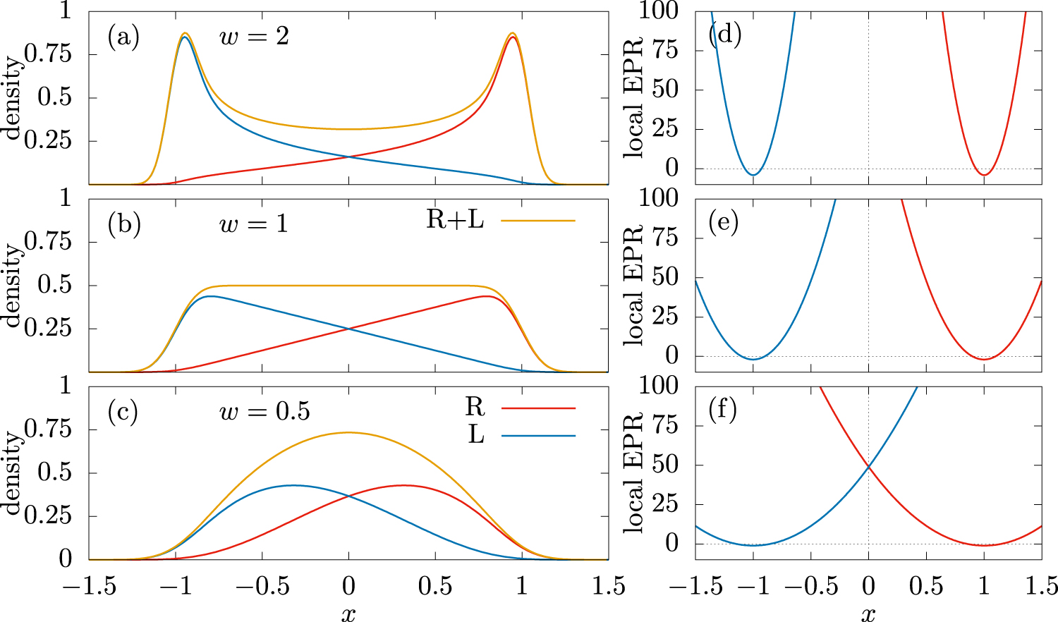
and σ_ψ (x) = σ_ϕ (−x) for left-moving particles, see figure 3. The local entropy production rate σ_ϕ is minimal at the characteristic point ξ = w/k, where a right-moving particle has a zero expected velocity because the self-propulsion equals the force exerted by the potential, and its motion is entirely due to the thermal noise. We can calculate (39) using the moments derived in section 2.3. On the basis of equation (28), the total stationary internal entropy production is

$$\begin{equation}{\dot {S}}_{i}=\frac{\alpha {w}^{2}}{D\left(k+\alpha \right)},\end{equation} \tag{ 41 }$$

see figure 4.

Zoom In Zoom Out Reset image size

Zoom In Zoom Out Reset image size

In this paper we have used the Doi-Peliti framework to describe an RnT particle in a harmonic potential and calculate its entropy production (41) and other observables (such as (24), (28), (F.4), (G.4), (H.2), (I.3), (D.3) and (D.7)) in closed form. The key result in equation (41) shows that the stationary internal entropy production of an RnT particle is proportional to that of a drift-diffusive particle in free space, where ${\dot {S}}_{i}={w}^{2}/D$ [46]. In the presence of an external harmonic potential (k > 0), the entropy production is always smaller than that of a free particle. If there is no tumbling (α = 0), then the system is an Ornstein–Uhlenbeck process, which is at equilibrium and therefore produces no entropy.

The positive entropy production rate implies the breaking of time symmetry whereby forward and backward trajectories are distinguishable [46]. This is visible in the trajectory of an RnT particle, such as in figure 1, where we can see that the particle runs fast when 'going down' the potential and it slows down as it moves up the steep slope of the potential.

Deriving the Doi-Peliti field theory of an RnT particle in a harmonic potential presents an important technical challenge. Due to the external harmonic potential, the action functional is semi-local both in real space and in Fourier space. Instead, to diagonalise the action we decomposed the fields in a basis of Hermite polynomials following the spirit of the harmonic oscillator [43].

Extending the above results to higher dimensions requires the tumbling mechanism to be suitably changed. The different spatial dimensions decouple only if tumbling between two velocities is maintained in each spatial direction. Otherwise, different mechanisms, such as a diffusive director as in active Brownian particles or RnT with the new direction taken from a uniform distribution [17, 24], require different approaches. In general it will no longer be possible to decompose the particle densities into scalar densities and polarities, which may need to be cast into a vector field. It is a matter of future research to find a convenient, microscopic field theory of RnT in higher dimensions.

The present example of an RnT particle illustrates the power of field theories that capture the microscopic dynamics to deal with active systems. Since the large scale behaviour of an RnT particle is that of a diffusive particle, by studying an effective theory that captures the large scale only, we would obtain a zero entropy production rate, in contradiction with our result (41). A similar coarse-graining simplification is assumed, for instance, when motility induced phase separation is modelled via quorum sensing, that is the self-propulsion depends on the particle density [24], instead of pairwise repulsive interactions.

Our work can be extended to studying Active Ornstein–Uhlenbeck Particles [44], whose self-propulsion is modelled by an Ornstein–Uhlenbeck process, and therefore share important features with an RnT particle in a harmonic potential. In particular, the field decomposition is also based on Hermite polynomials. Another extension for possible future work is to include a birth and death, or branching dynamics, by adding $\int \mathrm{d}x\enspace \enspace \mathrm{d}t\enspace \left\{r\tilde {\phi }\phi -{q}_{2}{\tilde {\phi }}^{2}\phi \right\}$ to the action (4) [55].

To study a microscopic description of motility induced phase separation, we can introduce pairwise interactions. Interactions between particles at positions x and y mediated by a potential V(x − y) result in the following term in the action

$$\begin{align}{\mathcal{A}}_{2}& =\int \mathrm{d}x\enspace \enspace \mathrm{d}y\enspace \enspace \mathrm{d}t\enspace \left({\partial }_{x}\tilde {\phi }\left(x,t\right)\phi \left(x,t\right)+{\partial }_{x}\tilde {\psi }\left(x,t\right)\psi \left(x,t\right)\right){V}^{\prime }\left(x-y\right)\\ & \quad {\times}\left(\left(\tilde {\phi }\left(y,t\right)+1\right)\phi \left(y,t\right)+\left(\tilde {\psi }\left(y,t\right)+1\right)\psi \left(y,t\right)\right),\end{align} \tag{ 42 }$$

which probes for the particle numbers of either species at a distance x − y and implements their interaction via the potential V. In terms of density and polarity fields, this nonlinear term is

$$\begin{align}{\mathcal{A}}_{2}& =\int \mathrm{d}x\enspace \enspace \mathrm{d}y\enspace \enspace \mathrm{d}t\enspace \left({\partial }_{x}\tilde {\rho }\left(x,t\right)\rho \left(x,t\right)+{\partial }_{x}\tilde {\nu }\left(x,t\right)\nu \left(x,t\right)\right){V}^{\prime }\left(x-y\right)\\ & \quad {\times}\left(\left(\tilde {\rho }\left(y,t\right)+1\right)\rho \left(y,t\right)+\tilde {\nu }\left(y,t\right)\nu \left(y,t\right)\right).\end{align} \tag{ 43 }$$

Having established the field-theoretic foundational work for an RnT particle, we shall now proceed to studying more intricate processes that will advance our understanding of active matter.

We would like to thank Umut Özer for his contribution to an earlier exploration on the field theory of an RnT particle in a harmonic potential. We are grateful to Ziluo Zhang for many enlightening discussions about the field theory of an RnT particle in two dimensions. We would also like to thank Marius Bothe, Benjamin Walter, Zigan Zhen, Luca Cocconi, Frédéric van Wijland, Julien Tailleur, Yuting Irene Li, Patrick Pietzonka and Davide Venturelli for fruitful discussions. This work was funded in part by the European Research Council under the EU's Horizon 2020 Programme, Grant No. 740269.

The formalism presented in section 2 can be generalised to anisotropic self-propulsion and asymmetric tumbling rates, which has applications in the context of gene regulation [29–32]. First, we consider the case where the self-propulsion velocities are w + Ω for right-moving particles and −w + Ω for left-moving particles, similar to a persistent random walk [56, 57]. The coupled Fokker–Planck equations in (3) then read

$$\begin{equation}{\partial }_{t}{P}_{\phi }=-{\partial }_{x}\left[\left(-kx+w+{\Omega}\right){P}_{\phi }\right]+D{\partial }_{x}^{2}{P}_{\phi }+\frac{\alpha }{2}\left({P}_{\psi }-{P}_{\phi }\right),\end{equation} \tag{ A.1 }$$

$$\begin{equation}{\partial }_{t}{P}_{\psi }=-{\partial }_{x}\left[\left(-kx-w+{\Omega}\right){P}_{\psi }\right]+D{\partial }_{x}^{2}{P}_{\psi }+\frac{\alpha }{2}\left({P}_{\phi }-{P}_{\psi }\right).\end{equation} \tag{ A.2 }$$

We see that the shift in the self-propulsion can be absorbed into the position x through the change

$$\begin{equation}x\to x-\frac{{\Omega}}{k},\end{equation} \tag{ A.3 }$$

so that we recover the Fokker–Planck equations in (3). Asymmetric velocities, Ω ≠ 0, therefore amount to a shift of the origin by Ω/k in the results above.

Second, assuming that the tumbling rates are α_ϕ = α + Λ and α_ψ = α − Λ, the Fokker–Planck equations in (3) read

$$\begin{equation}{\partial }_{t}{P}_{\phi }=-{\partial }_{x}\left[\left(-kx+w\right){P}_{\phi }\right]+D{\partial }_{x}^{2}{P}_{\phi }+\frac{\alpha +{\Lambda}}{2}\left({P}_{\psi }-{P}_{\phi }\right),\end{equation} \tag{ A.4 }$$

$$\begin{equation}{\partial }_{t}{P}_{\psi }=-{\partial }_{x}\left[\left(-kx-w\right){P}_{\psi }\right]+D{\partial }_{x}^{2}{P}_{\psi }+\frac{\alpha -{\Lambda}}{2}\left({P}_{\phi }-{P}_{\psi }\right),\end{equation} \tag{ A.5 }$$

so that the action functional in (4) aquires an additional bilinear term with coupling Λ,

$$\begin{align}\mathcal{A}& =\int \mathrm{d}x\enspace \enspace \mathrm{d}t\enspace \left\{\tilde {\phi }\left({\partial }_{t}\phi +{\partial }_{x}\left[\left(-kx+w\right)\phi \right]-D{\partial }_{x}^{2}\phi \right)\right.\\ & \quad +\tilde {\psi }\left({\partial }_{t}\psi +{\partial }_{x}\left[\left(-kx-w\right)\psi \right]-D{\partial }_{x}^{2}\psi \right)\\ & \quad \left.+\frac{\alpha }{2}\left(\tilde {\phi }-\tilde {\psi }\right)\left(\phi -\psi \right)+\frac{{\Lambda}}{2}\left(\tilde {\phi }+\tilde {\psi }\right)\left(\phi -\psi \right)\right\}.\end{align} \tag{ A.6 }$$

Along the lines of the derivation in section 2, we transform the fields to $\rho =\left(\phi +\psi \right)/\sqrt{2}$ and $\nu =\left(\phi -\psi \right)/\sqrt{2}$, and use the parametrisation in (11). It turns out that the additional bilinear term is local and hence it can be included in the Gaussian part,

$$\begin{align}{\mathcal{A}}_{0}& =\frac{1}{{L}^{2}}\sum\limits _{n,m}L{\delta }_{n,m}\int \mathrm{d}\hspace{-1pt}\bar\;\omega \enspace \enspace \mathrm{d}\hspace{-1pt}\bar{\;\omega }^{\prime }\enspace \delta \hspace{-2.5pt}\bar\;\left(\omega +{\omega }^{\prime }\right)\left[\left(-\mathring{{\imath}}\omega +kn\right){\tilde {\rho }}_{n}\left({\omega }^{\prime }\right){\rho }_{m}\left(\omega \right)\right.\\ & \quad +\left.\left(-\mathring{{\imath}}\omega +kn+\alpha \right){\tilde {\nu }}_{n}\left({\omega }^{\prime }\right){\nu }_{m}\left(\omega \right)+{\Lambda}{\tilde {\rho }}_{n}\left({\omega }^{\prime }\right){\nu }_{m}\left(\omega \right)\right].\end{align} \tag{ A.7 }$$

This new term results in the new bare propagator

instead of (16b) whereas the bare propagators ${\langle {\rho }_{n}\left(\omega \right){\tilde {\rho }}_{m}\left({\omega }^{\prime }\right)\rangle }_{0}$, ${\langle {\nu }_{n}\left(\omega \right){\tilde {\nu }}_{m}\left({\omega }^{\prime }\right)\rangle }_{0}$ and ${\langle {\rho }_{n}\left(\omega \right){\tilde {\nu }}_{m}\left({\omega }^{\prime }\right)\rangle }_{0}$ in (15) and (16a) remain unchanged.

The new contribution to the bare theory parametrised by Λ > 0 makes the diagram bookkeeping much more convoluted, although it is doable in principle. We leave it for future study, as it is beyond the scope of the present work.

The definition of Hermite polynomials according to the 'probabilists' convention' [58] we use in this paper is

$$\begin{equation}{H}_{n}\left(x\right)={\left(-1\right)}^{n}\enspace {e}^{\frac{{x}^{2}}{2}}\enspace \frac{{\mathrm{d}}^{n}}{\mathrm{d}{x}^{n}}\left({e}^{-\frac{{x}^{2}}{2}}\right),\end{equation} \tag{ B.1 }$$

where $x\in \mathbb{R}$, $n\in \mathbb{N}\cup \left\{0\right\}$. Some of the properties of Hermite polynomials that we use are listed in the following [58].

Orthogonality: Hermite polynomials are orthogonal with respect to the weight function $f\left(x\right)=\mathrm{exp} \left(-{x}^{2}/2\right)$,

$$\begin{equation}{\int }_{-\infty }^{\infty } \mathrm{d}x\enspace \enspace {e}^{-\frac{{x}^{2}}{2}}{H}_{n}\left(x\right){H}_{m}\left(x\right)=\sqrt{2\pi }\enspace n!\enspace {\delta }_{n,m},\end{equation} \tag{ B.2 }$$

where δ_n,m is the Kronecker delta.

Hermite's differential equation: Hermite polynomials ${H}_{n}\left(x\right)$ are eigenfunctions of the differential operator

$$\begin{equation}{H}^{{\prime\prime}}-x{H}^{\prime }=-\mu H,\end{equation} \tag{ B.3 }$$

for non-negative integer eigenvalues μ_n = n. Using this equation, we can show that the functions ${u}_{n}\left(x\right)=f\left(x/L\right){H}_{n}\left(x/L\right)$ are solution to the eigenvalue problem $\mathcal{L}\left[u\right]={u}^{\prime \prime }+{\left(x\enspace u\right)}^{\prime }/{L}^{2}=\lambda u$ in section 2, equation (7), with eigenvalues λ_n = −n/L² [59].

Generating function: Hermite polynomials can be obtained through the generating function

$$\begin{equation}{e}^{x\beta -\frac{1}{2}{\beta }^{2}}=\sum\limits _{n=0}^{\infty }{H}_{n}\left(y\right)\frac{{\beta }^{n}}{n!},\end{equation} \tag{ B.4 }$$

from which it follows that Hermite polynomials conform an Appell sequence, namely, they have the property

$$\begin{equation}{H}_{n}^{\prime }\left(x\right)=n{H}_{n-1}\left(x\right).\end{equation} \tag{ B.5 }$$

Recurrence relation: Hermite polynomials satisfy the recurrence relation

$$\begin{equation}{H}_{n+1}\left(x\right)=x{H}_{n}\left(x\right)-{H}_{n}^{\prime }\left(x\right).\end{equation} \tag{ B.6 }$$

Mehler's formula: Hermite polynomials satisfy the following identity [43, 58],

$$\begin{equation}\enspace {e}^{-\frac{{x}^{2}}{2}}\sum\limits _{n=0}^{\infty }\frac{{s}^{n}}{n!}{H}_{n}\left(x\right){H}_{n}\left(y\right)=\frac{1}{\sqrt{1-{s}^{2}}}\enspace {e}^{-\frac{{\left(x-ys\right)}^{2}}{2\left(1-{s}^{2}\right)}}.\end{equation} \tag{ B.7 }$$

We list the propagators that we have used to calculate in the observables. Using the bare propagators in (15) and the interaction part of the action in (12b), we obtain the following propagators in real time,

after letting r → 0. These propagators are then used to calculate the full propagator in real space via

$$\begin{equation}\langle \rho \left(x,t\right)\tilde {\rho }\left({x}^{\prime },{t}^{\prime }\right)\rangle =\frac{1}{{L}^{2}}\sum\limits _{n,m,N}{u}_{n}\left(x\right){\tilde {u}}_{m}\left({x}^{\prime }\right)\frac{1}{N!}{\left\langle {\rho }_{n}\left(t\right){\tilde {\rho }}_{m}\left({t}^{\prime }\right){\left(-{\mathcal{A}}_{1}\right)}^{N}\right\rangle }_{0},\end{equation} \tag{ C.7 }$$

where $\left(\sim \right){\rho }$ may be replaced by $\left(\sim \right){\nu }$. The stationary distribution is derived from this expression in appendix D.

The distribution of an RnT particle is captured by the propagator $P\left(x,t\right)=\langle \left(\phi \left(x,t\right)+\psi \left(x,t\right)\right)\tilde {\phi }\left({x}_{0},0\right)\rangle$, where the system is initialised at t₀ = 0 with a right-moving particle at x₀ [27, 60]. Diagrammatically, the particle distribution is

When Fourier transforming back into direct time, all poles $-\mathring{{\imath}}p$ of all bare propagators of the form ${\left(-\mathring{{\imath}}\omega +p\right)}^{-1}$, equation (15), eventually feature in the form $\mathrm{exp} \left(-pt\right)$. In the limit t → ∞, from equations (22a) and (22b), we have that any diagram containing $\tilde {\nu }$ as the right, incoming leg , decays exponentially in time t (see for instance (C.2), (C.3) and (C.6)). Moreover, the diagrams that have as their right, incoming leg decay exponentially with rate mk, so only those with m = 0 remain in the limit t → ∞. Then, the distribution in (D.1) reduces to

where the sum has contributions only from even n (see equations (21) and (23a)). The stationary distribution then reads

$$\begin{align}P\left(x\right)& =\underset{t\to \infty }{\mathrm{lim}}\enspace P\left(x,t\right)\\ & =\sqrt{\frac{k}{2\pi D}}\enspace {e}^{-\frac{k{x}^{2}}{2D}}\left(1+\sum\limits _{\begin{subarray}{c}n=2\\ n\;\text{even}\end{subarray}}^{\infty }{\left(\frac{w}{\sqrt{kD}}\right)}^{n}{H}_{n}\left(\sqrt{\frac{k}{D}}x\right)\prod\limits _{j=1}^{n}\frac{1}{j+{p}_{j}/k}\right),\end{align} \tag{ D.3 }$$

where p_j = α if j odd and p_j = r → 0 otherwise, see figures 3 and D1 ⁴ [29].

Similarly, the stationary distribution of a right-moving particle is

whose contribution is known from (D.3). As above, only diagrams that have index m = 0 remain in the limit t → ∞, so that

which has contributions only from odd n, see equations (22c) and (23d). Equation (D.6) has the same form as (D.3) except that the dummy variable n is odd. Therefore, the probability distribution in (D.5) contains the sum over both even and odd indices n ⩾ 0,

$$\begin{equation}\underset{t\to \infty }{\mathrm{lim}}\enspace {P}_{\phi }\left(x,t\right)=\frac{1}{2}\sqrt{\frac{k}{2\pi D}}\enspace {e}^{-\frac{k{x}^{2}}{2D}}\left(1+\sum\limits _{n=1}^{\infty }{\left(\frac{w}{\sqrt{kD}}\right)}^{n}{H}_{n}\left(\sqrt{\frac{k}{D}}x\right)\prod\limits _{j=1}^{n}\frac{1}{j+{p}_{j}/k}\right),\end{equation} \tag{ D.7 }$$

see figure 3 [29]. Alternatively, the stationary distributions (D.3) and (D.7) can in principle be derived from the Fokker–Planck equation (3) by inserting the ansatz $P\left(x\right)={\sum }_{n}{c}_{n}\enspace \mathrm{exp} \left(-k{x}^{2}/\left(2D\right)\right){H}_{n}\left(\sqrt{k/D}x\right)$ and determining the coefficients c_n recursively.

The entropy calculated in equation (41) is based on the Markovian evolution of the particle in terms of its position and species. However, Seifert's formulation of the entropy production [54, 65–67]

$$\begin{equation}{\mathring{\mathcal{S}}}_{i}=\underset{t\to \infty }{\mathrm{lim}}\enspace \frac{1}{t}\left\langle \mathrm{ln}\enspace \frac{p\left[x\left({t}^{\prime }\right)\right]}{p\left[{x}^{R}\left({t}^{\prime }\right)\right]}\right\rangle =\underset{t\to \infty }{\mathrm{lim}}\enspace \frac{1}{t}\int \mathcal{D}\left[x\right]p\left[x\left({t}^{\prime }\right)\right]\mathrm{ln}\left(\frac{p\left[x\left({t}^{\prime }\right)\right]}{p\left[{x}^{R}\left({t}^{\prime }\right)\right]}\right),\end{equation} \tag{ E.1 }$$

where p[x(t)] refers to the probability of observing a path x(t') for t' ∈ [0, t] and p[x^R (t')] to the probability of the reverse path to occur, allows for 'non-Markovian paths', i.e. paths not specified in a degree of freedom in which the process is Markovian. As a result, transition probabilities do not factorise, so that the path probabilities are not simply products, which makes them more difficult to calculate and manipulate. In the present case, we consider the evolution of the RnT particle system solely in terms of the particle's position. This is of particular relevance where the entropy production is used as a proxy for the particle's energy output that can be harvested. While we have made some progress, the derivation is incomplete and will need to be explored in future work.

RnT particles produce entropy even when their species is not known, which is visible in the apparent difference of forward and backward path probabilities. This is most easily seen in paths that reach from x = −ξ = −w/k to x = ξ and vice versa, figure 1, as forward paths show particles that move initially fast and slow down as they reach their destination, while backwards paths show a slow descent and a fast ascent. This difference is in marked contrast to RnT particles on a ring whose backward and forward trajectories are indistinguishable if their species and thus preferred direction is unknown.

To motivate the following, we first consider the probabilities of a path in terms of species and position x(t) probed at equidistant times t_i = iτ with i = 0, ..., N and x(t₀) = x₀. At stationarity, this amounts to creating particles with stationary probabilities P(x), equation (D.3), along the real line and then probing for the presence of a particle of suitable species at the desired positions. To simplify the notation, we consider at first only one species. The probability of a path is then

$$\begin{align}& \left\langle \prod\limits _{i=1}^{N}\left({\phi }^{{\dagger}}\left(x\left({t}_{i}\right),{t}_{i}\right)\phi \left(x\left({t}_{i}\right),{t}_{i}\right)\right)\int \mathrm{d}{x}_{0}\enspace P\left({x}_{0}\right){\phi }^{{\dagger}}\left({x}_{0},{t}_{0}\right)\right\rangle \\ & \hspace{25.0pt}=\int \mathrm{d}{x}_{0}\enspace P\left({x}_{0}\right)\prod\limits _{i=1}^{N}\left\langle \phi \left(x\left({t}_{i}\right),\tau \right)\tilde {\phi }\left(x\left({t}_{i-1}\right),0\right)\right\rangle ,\end{align} \tag{ E.2 }$$

where we have replaced $\left\langle \phi \left(x\left({t}_{i}\right),{t}_{i}\right)\tilde {\phi }\left(x\left({t}_{i-1}\right),{t}_{i-1}\right)\right\rangle$ by $\left\langle \phi \left(x\left({t}_{i}\right),\tau \right)\tilde {\phi }\left(x\left({t}_{i-1}\right),0\right)\right\rangle$, because of time-homogeneity.

The path probabilities to be used in equation (E.1) are sums over all contributions from the particle being any of the species at any point in time. The particle number operator ϕ^† ϕ in equation (E.2) therefore needs to be replaced by ϕ^† ϕ + ψ^† ψ = ρ^† ρ + ν^† ν. This can be expressed most comprehensively using a transfer matrix,

$$\begin{align}p\left(\left[x\left(t\right)\right]\right)& =\int \mathrm{d}{x}_{0}\enspace {\left(\begin{matrix}\hfill 1\hfill \\ \hfill 1\hfill \end{matrix}\right)}^{\mathrm{T}}\\ & \quad \cdot \prod\limits _{i=1}^{N}\left(\begin{matrix}\hfill \left\langle \phi \left(x\left({t}_{i}\right),\tau \right)\tilde {\phi }\left(x\left({t}_{i-1}\right),0\right)\right\rangle \hfill & \hfill \left\langle \phi \left(x\left({t}_{i}\right),\tau \right)\tilde {\psi }\left(x\left({t}_{i-1}\right),0\right)\right\rangle \hfill \\ \hfill \left\langle \psi \left(x\left({t}_{i}\right),\tau \right)\tilde {\phi }\left(x\left({t}_{i-1}\right),0\right)\right\rangle \hfill & \hfill \left\langle \psi \left(x\left({t}_{i}\right),\tau \right)\tilde {\psi }\left(x\left({t}_{i-1}\right),0\right)\right\rangle \hfill \end{matrix}\right)\left(\begin{matrix}\hfill {P}_{\phi }\left({x}_{0}\right)\hfill \\ \hfill {P}_{\psi }\left({x}_{0}\right)\hfill \end{matrix}\right)\end{align} \tag{ E.3 }$$

and correspondingly in terms of fields ρ and ν. The probability P_ϕ (x₀) denotes the stationary density of finding a particle of species ϕ at x₀ and correspondingly for ψ, see (D.7).

Using the short-time propagators in equations (24) and (25), and variations thereof obtained by replacing w by −w, results for the transfer matrix in equation (E.3)

$$\begin{align}M\left(x\to y;\tau \right)& =\left(\begin{matrix}\hfill \left\langle \phi \left(y,\tau \right)\tilde {\phi }\left(x,0\right)\right\rangle \hfill & \hfill \left\langle \phi \left(y,\tau \right)\tilde {\psi }\left(x,0\right)\right\rangle \hfill \\ \hfill \left\langle \psi \left(y,\tau \right)\tilde {\phi }\left(x,0\right)\right\rangle \hfill & \hfill \left\langle \psi \left(y,\tau \right)\tilde {\psi }\left(x,0\right)\right\rangle \hfill \end{matrix}\right)\\ & =\frac{1}{\sqrt{4\pi D\tau }}\enspace {e}^{-\frac{{\left(y-x\left(1-k\tau \right)\right)}^{2}}{4D\tau }}\\ & \quad {\times}\left(\begin{matrix}\hfill \mathrm{exp} \left(\frac{w\left(y-x+kx\tau \right)}{2D}-\frac{\alpha }{2}\tau \right)\hfill & \hfill \frac{\alpha }{2}\tau \hfill \\ \hfill \frac{\alpha }{2}\tau \hfill & \hfill \mathrm{exp} \left(-\frac{w\left(y-x+kx\tau \right)}{2D}-\frac{\alpha }{2}\tau \right)\hfill \end{matrix}\right)\end{align} \tag{ E.4 }$$

where we have used expansions like

$$\begin{align}& 1+\frac{w\left(y-x\right)}{2D}+\left(-\frac{\alpha }{2}+\frac{w}{4D}\left(k\left(y+x\right)-\alpha \left(y-x\right)\right)\right)\tau +\mathcal{O}\left({\tau }^{2}\right)\\ & \hspace{25.0pt}=\mathrm{exp} \left(\frac{w\left(y-x+kx\tau \right)}{2D}-\frac{\alpha }{2}\tau \right)\left(1+\mathcal{O}\left({\tau }^{2}\right)\right),\end{align} \tag{ E.5 }$$

assuming that $y-x=\tau \dot {x}\in \mathcal{O}\left(\tau \right)$. The matrix product to determine in equation (E.3) is thus

$$\begin{equation}M\left(x\left({t}_{N-1}\right)\to x\left({t}_{N}\right);\tau \right)M\left(x\left({t}_{N-2}\right)\to x\left({t}_{N-1}\right);\tau \right)\dots M\left(x\left({t}_{0}\right)\to x\left({t}_{1}\right);\tau \right)\end{equation} \tag{ E.6 }$$

which may be approximated by writing

$$\begin{equation}M\left(x\to y;\tau \right)=\frac{1}{\sqrt{4\pi D\tau }}\enspace {e}^{-\frac{{\left(\dot {x}+xk\right)}^{2}}{4D}\tau }\enspace \mathrm{exp} \left(\left(\begin{matrix}\hfill \frac{w\left(\dot {x}+kx\right)}{2D}-\frac{\alpha }{2}\hfill & \hfill \frac{\alpha }{2}\hfill \\ \hfill \frac{\alpha }{2}\hfill & \hfill -\frac{w\tau \left(\dot {x}+kx\right)}{2D}-\frac{\alpha }{2}\hfill \end{matrix}\right)\tau \right)+\mathcal{O}\left({\tau }^{2}\right)\end{equation} \tag{ E.7 }$$

using the shorthand $\dot {x}\tau =y-x$ and $\dot {x}\left({t}_{i}\right)\tau =x\left({t}_{i+1}\right)-x\left({t}_{i}\right)$ below. To our understanding, no grave error is introduced at this stage by omitting terms $\mathcal{O}\left({\tau }^{2}\right)$. Much of the derivation above can be made keeping the Hermite basis used for the propagators (15), which immediately results in a matrix exponential, as the Fourier transform of the inverse matrix ${\left(-\mathring{{\imath}}\omega \mathbf{1}-F\right)}^{-1}$ is the matrix $\mathrm{exp} \left(\tau F\right)$ [38] (also appendix C).

To ease notation, we may write

$$\begin{equation}M\left(x\to y;\tau \right)=\frac{1}{\sqrt{4\pi D\tau }}\enspace {e}^{-\frac{{\left(\dot {x}+xk\right)}^{2}}{4D}\tau }\enspace {e}^{m\left(x\to y;\tau \right)}\end{equation} \tag{ E.8 }$$

with suitable exponentiated matrix m(x → y; τ) in the following. What seems to undermine further progress to calculate the matrix product in equation (E.3) is that the product $\mathrm{exp} \left(m\left(y\to z;\tau \right)\right)\mathrm{exp} \left(m\left(x\to y;\tau \right)\right)$ can be written as the exponential of the sum, $\mathrm{exp} \left(m\left(y\to z;\tau \right)+m\left(x\to y;\tau \right)\right)$ only when the matrices m(x → y; τ) and m(y → z; τ) commute. Yet they generally do not, with correction terms of the form

$$\begin{align}& \mathrm{exp} \left(m\left(x\left({t}_{N-1}\right)\to x\left({t}_{N}\right);\tau \right)\right)\mathrm{exp} \left(m\left(x\left({t}_{N-2}\right)\to x\left({t}_{N-1}\right);\tau \right)\right)\\ & \hspace{25.0pt}=\mathrm{exp} \left(m\left(x\left({t}_{N-1}\right)\to x\left({t}_{N}\right);\tau \right)+m\left(x\left({t}_{N-2}\right)\to x\left({t}_{N-1}\right);\tau \right)\right)\\ & \quad \hspace{25.0pt}+\frac{{\tau }^{2}}{2}\left(\begin{matrix}\hfill 0\hfill & \hfill \frac{wk\alpha }{2D}\left(x\left({t}_{N-1}\right)-x\left({t}_{N-2}\right)\right)\hfill \\ \hfill -\frac{wk\alpha }{2D}\left(x\left({t}_{N-1}\right)-x\left({t}_{N-2}\right)\right)\hfill & \hfill 0\hfill \end{matrix}\right).\end{align} \tag{ E.9 }$$

Proceeding on the basis of the Trotter formula, we find in the continuum limit τ → 0

$$\begin{align}p\left(\left[x\left(t\right)\right]\right)& ={\mathcal{N}}^{-1}\enspace {e}^{-\frac{1}{4D}{\int }_{0}^{t}\mathrm{d}{t}^{\prime }\enspace {\left(\dot {x}\left({t}^{\prime }\right)+kx\left({t}^{\prime }\right)\right)}^{2}}\int \mathrm{d}{x}_{0}\enspace {\left(\begin{matrix}\hfill 1\hfill \\ \hfill 1\hfill \end{matrix}\right)}^{\mathrm{T}}\\ & \quad \cdot \mathrm{exp} \left({\int }_{0}^{t} \mathrm{d}{t}^{\prime }\enspace \left(\begin{matrix}\hfill \frac{w}{2D}\left(\dot {x}\left({t}^{\prime }\right)+kx\left({t}^{\prime }\right)\right)-\frac{\alpha }{2}\hfill & \hfill \frac{\alpha }{2}\hfill \\ \hfill \frac{\alpha }{2}\hfill & \hfill -\frac{w}{2D}\left(\dot {x}\left({t}^{\prime }\right)+kx\left({t}^{\prime }\right)\right)-\frac{\alpha }{2}\hfill \end{matrix}\right)\right)\\ & \quad \cdot \left(\begin{matrix}\hfill {P}_{\phi }\left({x}_{0}\right)\hfill \\ \hfill {P}_{\psi }\left({x}_{0}\right)\hfill \end{matrix}\right),\end{align} \tag{ E.10 }$$

with suitable normalisation ${\mathcal{N}}^{-1}$. Equation (E.10) can be simplified further by noting that any term of the form ${\int }_{0}^{t} \mathrm{d}{t}^{\prime }\enspace \enspace \dot {x}\left({t}^{\prime }\right)=x\left(t\right)-x\left(0\right)$ or ${\int }_{0}^{t} \mathrm{d}{t}^{\prime }\enspace \enspace x\left({t}^{\prime }\right)\dot {x}\left({t}^{\prime }\right)/2={x}^{2}\left(t\right)-{x}^{2}\left(0\right)$ will be dominated by other terms of order $\mathcal{O}\left(t\right)$ as the particle is in a binding potential, so that x(t) − x(0) and x²(t) − x²(0) are essentially bounded. We may thus replace at any stage ${\int }_{0}^{t} \mathrm{d}{t}^{\prime }\enspace {\left(\dot {x}\left({t}^{\prime }\right)+kx\left({t}^{\prime }\right)\right)}^{2}$ by ${\int }_{0}^{t} \mathrm{d}{t}^{\prime }\enspace \enspace {\dot {x}}^{2}\left({t}^{\prime }\right)+{\left(kx\left({t}^{\prime }\right)\right)}^{2}$ and similarly inside the matrix, so that

$$\begin{align}p\left(\left[x\left(t\right)\right]\right)& ={\mathcal{N}}^{-1}\enspace {e}^{-\frac{1}{4D}{\int }_{0}^{t} \mathrm{d}{t}^{\prime }\enspace \left({\dot {x}}^{2}\left({t}^{\prime }\right)+k{x}^{2}\left(t\right)\right)}\int \mathrm{d}{x}_{0}\enspace {\left(\begin{matrix}\hfill 1\hfill \\ \hfill 1\hfill \end{matrix}\right)}^{\mathrm{T}}\\ & \quad \cdot \mathrm{exp} \left({\int }_{0}^{t} \mathrm{d}{t}^{\prime }\enspace \left(\begin{matrix}\hfill \frac{w}{2D}kx\left({t}^{\prime }\right)-\frac{\alpha }{2}\hfill & \hfill \frac{\alpha }{2}\hfill \\ \hfill \frac{\alpha }{2}\hfill & \hfill -\frac{w}{2D}kx\left({t}^{\prime }\right)-\frac{\alpha }{2}\hfill \end{matrix}\right)\right)\left(\begin{matrix}\hfill {P}_{\phi }\left({x}_{0}\right)\hfill \\ \hfill {P}_{\psi }\left({x}_{0}\right)\hfill \end{matrix}\right).\end{align} \tag{ E.11 }$$

This expression is invariant under $\dot {x}\to -\dot {x}$, i.e. forward and backward paths are incorrectly determined to have the same probability.

The apparent failure of the formalism is not resolved by considering the Ito-Stratonovich dilemma that occurs when writing

$$\begin{equation}\underset{\tau \to 0}{\mathrm{lim}}\sum\limits _{i}\left(x\left({t}_{i+1}\right)-x\left({t}_{i}\right)\right)x\left({t}_{i}\right)={\int }_{0}^{t} \mathrm{d}{t}^{\prime }\enspace \enspace \dot {x}\left({t}^{\prime }\right)x\left({t}^{\prime }\right)\end{equation} \tag{ E.12 }$$

rather than

$$\begin{align}& \underset{\tau \to 0}{\mathrm{lim}}\sum\limits _{i}\left(x\left({t}_{i+1}\right)-x\left({t}_{i}\right)\right)x\left({t}_{i}\right)\\ & \hspace{25.0pt}=\underset{\tau \to 0}{\mathrm{lim}}\sum\limits _{i}\left(x\left({t}_{i+1}\right)-x\left({t}_{i}\right)\right)\left(\frac{x\left({t}_{i+1}\right)+x\left({t}_{i}\right)}{2}-\frac{x\left({t}_{i+1}\right)-x\left({t}_{i}\right)}{2}\right)\\ & \hspace{25.0pt}={\int }_{0}^{t} \mathrm{d}{t}^{\prime }\enspace \enspace \frac{1}{2}\dot {x}\left({t}^{\prime }\right)x\left({t}^{\prime }\right).\end{align} \tag{ E.13 }$$

Remarkably, proceeding from equation (E.10) without removing integrals of the form $\int \mathrm{d}{t}^{\prime }\enspace \enspace \dot {x}$ and setting k → 0 seems to correctly produce the path probabilities for RnT on the ring. The resolution of the problems to determine the path probabilities encountered above is an interesting question to pursue in future research.

The mean square displacement is defined as

$$\begin{equation}{R}^{2}\left(t\right)=\left\langle {\left(x\left(t\right)-{x}_{0}\right)}^{2}\right\rangle .\end{equation} \tag{ F.1 }$$

Assuming that the system is initialised with a right-moving particle, the propagator that probes for any particle at a later time is $\left\langle \left(\phi \left(x,t\right)+\psi \left(x,t\right)\right)\tilde {\phi }\left({x}_{0},0\right)\right\rangle$. Following the same scheme as in section 2.3, the first and second moments of the position of an RnT particle are

$$\begin{equation}\left\langle x\left(t\right)\right\rangle ={x}_{0}\enspace {e}^{-kt}+\frac{w}{k-\alpha }\left({e}^{-\alpha t}-{e}^{-kt}\right),\end{equation} \tag{ F.2 }$$

$$\begin{align}\left\langle {x}^{2}\left(t\right)\right\rangle & ={x}_{0}^{2}\enspace {e}^{-2kt}+\frac{D}{k}\left(1-{e}^{-2kt}\right)+2\frac{{x}_{0}w}{k-\alpha }\left({e}^{-\left(k+\alpha \right)t}-{e}^{-2kt}\right)\\ & \quad +2{w}^{2}\left(\frac{\mathrm{exp} \left(-2kt\right)}{2k\left(k-\alpha \right)}+\frac{\mathrm{exp} \left(-\left(k+\alpha \right)t\right)}{\left(k+\alpha \right)\left(\alpha -k\right)}+\frac{1}{2k\left(k+\alpha \right)}\right).\end{align} \tag{ F.3 }$$

Then, the mean square displacement at stationarity is

$$\begin{equation}\underset{t\to \infty }{\mathrm{lim}}\enspace {R}^{2}\left(t\right)={x}_{0}^{2}+\frac{D}{k}+\frac{{w}^{2}}{k\left(k+\alpha \right)},\end{equation} \tag{ F.4 }$$

see figure F1(a).

Zoom In Zoom Out Reset image size

To calculate the expected velocity of a right-moving particle, one could naïvely differentiate the expected position $\left\langle {x}_{\phi }\left(t\right)\right\rangle$ in equation (27b) with respect to time,

$$\begin{equation}{\partial }_{t}\left\langle {x}_{\phi }\left(t\right)\right\rangle =\int \mathrm{d}x\enspace \enspace x{\partial }_{t}{P}_{\phi }\left(x,t\right).\end{equation} \tag{ G.1 }$$

However, this expression fails to capture the expected velocity because in the limit t → ∞, the stationary distribution satisfies ∂_t P_ϕ (x, t) = 0, implying that the result in (G.1) is zero. This seems in contradiction to the nature of an RnT particle, which has a perpetual non-zero drift even when 'stuck' at times. Ultimately, the ambiguity in the definition of the velocity is a matter of Ito versus Stratonovich, namely to consider a particle's displacement conditional to its point of departure (Ito), its point of arrival or the average of the two (Stratonovich).

The instantaneous velocity of a right-moving particle departing from x₀ can immediately be derived from its short-time propagator equation (24),

$$\begin{equation}{w}_{\phi }\left({x}_{0}\right)=\underset{\tau \to 0}{\mathrm{lim}}\frac{1}{\tau }\int \mathrm{d}y\enspace \left(y-{x}_{0}\right)\left\langle \phi \left(y,\tau \right)\tilde {\phi }\left({x}_{0},0\right)\right\rangle =w-k{x}_{0},\end{equation} \tag{ G.2 }$$

which in fact is the apparent velocity featuring in the Fokker–Planck equation (3a). The expected velocity of a right-moving particle $\left\langle {\mathcal{W}}_{\phi }\left(t\right)\right\rangle$ anywhere in the system at time t after having started at x₀ at time t₀ is therefore the conditional expectation

$$\begin{equation}\left\langle {\mathcal{W}}_{\phi }\left(t;{x}_{0}\right)\right\rangle =\frac{\int \mathrm{d}x\enspace \left(w-kx\right)\langle \phi \left(x,t\right)\tilde {\phi }\left({x}_{0},{t}_{0}\right)\rangle }{\int \mathrm{d}{x}^{\prime }\enspace \langle \phi \left({x}^{\prime },t\right)\tilde {\phi }\left({x}_{0},{t}_{0}\right)\rangle },\end{equation} \tag{ G.3 }$$

which, using equations (27a) and (27b), is, at stationarity

$$\begin{equation}\underset{t\to \infty }{\mathrm{lim}}\enspace \left\langle {\mathcal{W}}_{\phi }\left(t;{x}_{0}\right)\right\rangle =\frac{\alpha w}{k+\alpha },\end{equation} \tag{ G.4 }$$

see figure F1(b).

The two-point correlation function $\mathcal{F}\left(x,y;t\right)$ is the observable

$$\begin{align}\mathcal{F}\left(x,y;t\right)& =\left\langle \left(\phi \left(x,t\right)+\psi \left(x,t\right)\right)\left(\phi \left(y,t\right)+\psi \left(y,t\right)\right)\tilde {\phi }\left({x}_{0},0\right)\right\rangle \\ & \quad +\left\langle \left(\phi \left(x,t\right)+\psi \left(x,t\right)\right)\tilde {\phi }\left({x}_{0},0\right)\right\rangle \delta \left(x-y\right),\end{align} \tag{ H.1 }$$

where, after placing a right-moving particle at x₀ at time t₀, the system is probed for any particle at positions x and y simultaneously. The second term contributing only when x = y has its origin in the commutation relation of the creation and annihilation operators [39]. Since there is exactly one RnT particle in the system, it cannot be in two different positions at the same time and therefore $\mathcal{F}\left(x,y;t\right)=0$ for all t when x ≠ y. Diagrammatically, (H.1) may be written as

which is zero at x ≠ y due to a lack of a vertex , i.e. due to the impossibility of joining a single incoming leg with two out-going legs because there is no suitable vertex available. This is an example of how a Doi-Peliti field theory retains the particle entity. At x = y the two-point correlation function reduces to the propagators in equations (23a) and (23c).

The correlation function $\left\langle x\left(t\right)x\left({t}^{\prime }\right)\right\rangle$, with t₀ < t' < t, is given by the observable

$$\begin{equation}\left\langle x\left(t\right)x\left({t}^{\prime }\right)\right\rangle =\int \mathrm{d}x\enspace \enspace \mathrm{d}{x}^{\prime }\enspace \enspace x\enspace {x}^{\prime }\mathcal{G}\left(x,{x}^{\prime },{x}_{0};t,{t}^{\prime },{t}_{0}\right),\end{equation} \tag{ I.1 }$$

where the 'propagator' is now

$$\begin{align}\mathcal{G}\left(x,{x}^{\prime },{x}_{0};t,{t}^{\prime },{t}_{0}\right)& =\left\langle \left[\phi \left(x,t\right)+\psi \left(x,t\right)\right]\left[\tilde {\phi }\left({x}^{\prime },{t}^{\prime }\right)\phi \left({x}^{\prime },{t}^{\prime }\right)\right.\right.\\ & \quad +\left.\left.\tilde {\psi }\left({x}^{\prime },{t}^{\prime }\right)\psi \left({x}^{\prime },{t}^{\prime }\right)\right]\tilde {\phi }\left({x}_{0},{t}_{0}\right)\right\rangle .\end{align} \tag{ I.2 }$$

This propagator indicates that the system is initialised with a right-moving particle at x₀ at time t₀ = 0, and it is let to evolve by an interval of time t' − t₀. At time t', the propagator probes for the presence of a particle at x', which involves its annihilation and immediate re-creation. The system is then let to evolve a further interval of time t − t', at which point the presence of either species is measured again at position x. Following the same procedure as in section 2.3, the two-time correlation function reads

$$\begin{align}\left\langle x\left(t\right)x\left({t}^{\prime }\right)\right\rangle & =\enspace {e}^{-k\left(t-{t}^{\prime }\right)}\left[{x}_{0}^{2}\enspace {e}^{-2k{t}^{\prime }}+\frac{D}{k}\left(1-{e}^{-2k{t}^{\prime }}\right)+2\frac{{x}_{0}w}{k-\alpha }\left({e}^{-\left(k+\alpha \right){t}^{\prime }}-{e}^{-2k{t}^{\prime }}\right)\right.\\ & \quad +\left.2{w}^{2}\left({e}^{-2k{t}^{\prime }}\frac{1}{2k\left(k-\alpha \right)}+{e}^{-\left(k+\alpha \right){t}^{\prime }}\frac{1}{\left(k+\alpha \right)\left(\alpha -k\right)}+\frac{1}{2k\left(k+\alpha \right)}\right)\right]\\ & \quad +\frac{w}{k+\alpha }\left(1-{e}^{-\left(k+\alpha \right)\left(t-{t}^{\prime }\right)}\right)\left[\frac{w}{k+\alpha }\left(1-{e}^{-\left(k+\alpha \right){t}^{\prime }}\right)+{x}_{0}\enspace {e}^{-\left(k+\alpha \right){t}^{\prime }}\right],\end{align} \tag{ I.3 }$$

see [22] for details.

Zoom In Zoom Out Reset image size