
Abstract
Spectral decomposition based on sparse constrained inversion, as proposed in recent years, is a high-resolution time-frequency domain analysis method. However, the traditional inverse spectral decomposition (ISD) algorithm is based on an inverse wavelet transform (IWT) whose mother wavelet is a Ricker wavelet function instead of an adaptive wavelet, which causes poor continuity and instability of the ISD results. In this paper, we have extended ISD into other linear transforms and have developed an ISD based on inverse S transform (ISD-IST), which has higher continuity and stability due to the more adjustable and adaptable mother wavelet of the S transform. Comparison of conventional methods and the ISD-IST shows that the ISD (ISD-IWT and ISD-IST) methods have higher resolution and accuracy and can provide more reliable time-frequency phase spectra, and it further verifies the greater continuity and stability of ISD-IST over ISD-IWT. Frequency-dependent AVO (FAVO) inversion is regarded as a potential hydrocarbon identification technique (Wilson et al 2009 SEG Technical Program Expanded Abstracts pp 341–5). However, it is frequency-decomposition based, which means that inversion results can be greatly affected by the effect of time-frequency analysis (Wu et al 2010 SEG Technical Program Expanded Abstracts pp 425–9; Wu et al 2014 Geophys. Prospect. 62 1224–37). Combining the FAVO inversion and high-resolution time-frequency decomposition ISD allows better dispersion attributes to be obtained. Results from application in Southwest China demonstrate that the high frequency-resolution of ISD is helpful in the extraction of gas-induced frequency anomalies from post-stack data, and its high time-resolution helps to obtain high time-resolution gas-induced dispersion results from FAVO inversion. The results of FAVO-ISD not only agree better with well information, but also supply more credible boundary information for the reservoirs. ISD-IST can provide more continuous results and smoother boundary information for the gas reservoir than ISD-IWT.
Export citation and abstract BibTeX RIS

Original content from this work may be used under the terms of the Creative Commons Attribution 3.0 licence. Any further distribution of this work must maintain attribution to the author(s) and the title of the work, journal citation and DOI.
1. Introduction
Due to the heterogeneity of the underground medium, the amplitude, frequency and phase of a seismic signal change with wave propagation—in other words, the seismic signal is a non-stationary signal. Thus, it is far from enough to analyze the non-stationary signal only in the time domain. Spectral decomposition technology provides joint distribution information for the time and frequency domains, and it can clearly describe the relationship between the frequency and time information in the signals.
The conventional methods of time-frequency analysis are divided into two categories, linear transform and bilinear transform. Linear transform is the most widely used time-frequency analysis method; it includes the short-time Fourier transform (STFT), the continuous wavelet transform (CWT), the S transform (ST) and the generalized ST (GST), and some improved methods. Gabor (1946) introduced the concept of the analytic signal (complex signal) into signal analysis, and proposed the STFT. In following years, signal analysis in time-frequency domains raised the interests of researchers and then a number of new methods were proposed. Morlet (1982) devised the CWT and applied it to seismic signal analysis. The CWT stimulates the development of non-stationary seismic signal analysis (Sinha et al 2005, Bi et al 2014). Based on the STFT and CWT, Stockwell et al (1996) put forward the ST. Then later workers (Gao et al 2003, Pinneger and Mansinha 2003) changed the window function of the ST and proposed the GST.
The bilinear transform methods are mainly the Wigner–Ville distribution (WVD) and its improved algorithms. The WVD was put forward by Ville (1948) based on the Wigner distribution, proposed by Wigner (1932). The WVD effectively solves the problem of the poor time-frequency focus induced by the non-adjustable window of STFT but it is limited by its cross terms. Many researchers tried to remove the cross terms to improve the accuracy of the signal analysis. Some reduced interference distributions, such as the pseudo WVD (PWVD) and the smoothed pseudo WVD (SPWVD), were proposed and applied in a different subject area (Auger and Flandrin 1995, Wu and Liu 2009, Wang et al 2012). These various improved WVD methods remove the interferences of the cross terms but to some extent reduce the time-frequency resolution of the decomposition results. Mallat and Zhang (1993) and Chakraborty and Okaya (1995) combined the matching pursuit (MP) and WVD to propose the MP-WVD method, which has a higher time-frequency resolution. Another drawback of WVD is that its time-frequency spectrum is real, and cannot be used for phase spectrum analysis.
The inverse spectral decomposition (ISD) is a relatively new method for time-frequency analysis. It is different from the previous two categories in that it obtains the spectral decomposition by solving the inverse problem (Portniaguine and Castagna 2004). The core work for solving it is to minimize the objective function which is a weighted sum of a misfit and a constraint item. In this process, the reverse wavelet transform serves as a forward operator. The inversion reconstructs the wavelet coefficients (time-frequency spectra) that not only represent the seismic data but also satisfy the constraint. The choice of the constraint is a matter of cardinal significance due to its important influence on the solution. By testing decompositions based on different constraints, Portniaguine and Castagna (2004) determined that the sparse spike solution has superior resolution in both time and frequency, and proposed to solve ISD with sparse inversion algorithms to derive a sparse time-frequency map. This problem can be solved as a basis pursuit (BP) problem or a BP de-noising problem (Han et al 2012). The spectral projected gradient for L1 minimization (SPGL1) (Ewout and Friedlander 2008) is reported as a fast method for such problems. Han et al (2012) introduced the SPGL1 algorithm into ISD to seek a sparse spectrum with superior higher resolution, and its application is effective in seismic de-noising. The sparse constrained ISD method can also be applied in other research fields.
Frequency-dependent attenuation and dispersion are attracting more and more interest because they are believed to be directly associated to rock properties and information on hydrocarbon saturation. Batzle et al (2001) noted that the velocities commonly vary across different frequency bands and the velocity dispersion will be influenced by fluid mobility within the pore spaces. Batzle et al (2006) found that the dominant factors for velocity dispersion seem to be the squirt flow, and the inverse relationship between characteristic frequency and fluid viscosity. Through numerical modeling analysis, Chapman et al (2006) found that there is a sharp increase in P-velocity dispersion between the high and low frequency limits, when water within pore space is substituted for gas. This has important implications: fluid induced velocity dispersion can result in frequency-dependent reflection coefficients and frequency-dependent AVO (FAVO).
Based on previous research involving dynamic rock physics models and the understanding of fluid-induced dispersion, Wilson et al (2009) and Wilson and Adam (2010) proposed FAVO inversion, a new potential method of extracting fluid-induced dispersion information directly from pre-stack data. The FAVO inversion technique raised a lot of attention from scholars and it is regarded as a potential hydrocarbon identification technique. Application of spectral decomposition techniques allows FAVO behavior due to fluid saturation to be detected in seismic data, because reflections from hydrocarbon-saturated zone are thought to have a tendency of being low frequency (Castagna et al 2003). Because the FAVO inversion is a frequency-decomposition based method, the result of the time-frequency analysis is of vital importance for the accuracy and robustness of estimating seismic dispersion. Wu et al (2010) compared three different spectral decomposition techniques and chose the one with highest resolution, the smoothed SPWVD, to combine with FAVO inversion. The greater application of spectral decomposition techniques allows the FAVO inversion to produce enhanced measures of dispersion. Therefore, a time-frequency analysis method with high resolution, high accuracy and high stability is needed for FAVO inversion. The previously mentioned sparse constrained ISD method produces high-resolution time-frequency maps which can be used with FAVO inversion to enhance the subsequent dispersion attributes and improve hydrocarbon detection.
Although the sparse spike solution helps ISD to derive a high-resolution time-frequency spectrum, it has a lower fault tolerance of the analysis results than other constraints, such as the L2 norm. It means that the existence of even a small difference induced by an inaccurate forward operator between the analysis results and the real spectrum will cause the sparse focused energy to locate at the wrong position while its real position shows very low or even no energy. This will subsequently cause low lateral continuity and stability of the iso-frequency section extracted from the time-frequency spectrum. The sparser the spectrum (corresponding to the higher-resolution time-frequency spectrum) we get, the lower continuity the frequency section may have. Therefore, an adaptive forward operator (inverse transform) is essential to reduce the difference between analysis results and the real spectrum, and hence improve the continuity. The more applicable the inverse transform we use, the better stability the inverse spectrum may have. The traditional ISD algorithm is based on IWT, whose mother wavelet is a Ricker wavelet instead of an adaptive wavelet, which causes poor continuity and stability of the frequency-component section of ISD-IWT. The subsequent FAVO inversion thus produces dispersion results with low continuity and stability. Therefore, we need an inverse transform with better adaptiveness to improve on this. The ST uses the adjustable Morlet wavelet as the mother wavelet, in which not only the wavelet scale can be adjusted but the local phase information can be retained (Stockwell et al 1996, Stockwell 2007). Theoretically speaking, an ISD based on the ST may be more applicable for the real data analysis of FAVO inversion.
In this paper, a detailed derivation of the ISD based on IWT (ISD-IWT) is given. Then we extend the ISD into the ST and set out the concept of the ISD based on the inverse ST (ISD-IST). By synthetic signal and real data tests, a comparison of traditional methods and ISD-IST is conducted, which demonstrates that the ISD-IST not only retains the high time- and frequency-resolution, but enhances the stability of the ISD and improves the continuity of the results. Because the FAVO inversion is frequency-decomposition based and inversion results can be greatly affected by the time-frequency analysis methods, we use high-resolution ISD in the FAVO inversion to calculate the dispersion attribute from pre-stack data. The application results demonstrate that the high time- and frequency-resolution of ISD is helpful to enhance the resolution of the inversion results and the credibility of the hydrocarbon prediction. The FAVO inversion based on ISD-IST is not only in better agreement with well information, but also supplies more credible boundary information on reservoirs because of its good continuity.
2. Improved ISD
2.1. Traditional ISD algorithm
The main idea of ISD is regarding the spectral decomposition as an inversion problem and solving it with sparse inversion algorithms to derive a sparse time-frequency map. In the process of solving the inverse problem, the inverse transform serves as the forward operator that is essential to the inversion. The traditional ISD algorithm uses the inverse wavelet transform (IWT) whose mother wavelet is a complex Ricker wavelet as its forward operator. Because the mother wavelet  (the Ricker wavelet) satisfies the admissibility condition, the wavelet transform has an inverse transform. The IWT can be expressed as:

where a is the scale factor, and b is the translation factor;  is the wavelet basis, also known as the mother wavelet. Formula (1) can be expressed as a convolution form

and a matrix form
where ![${X}_{a1}={X}_{a2}\,=\,\cdots \,=\,{X}_{am}=\left[\begin{array}{cccc}{x}_{t1} & {x}_{t2} & \cdots & {x}_{tn}\end{array}\right]$](https://content.cld.iop.org/journals/1742-2140/15/4/1446/revision2/jgeaab1d6ieqn3.gif) is a matrix with dimension
is a matrix with dimension  corresponding to a trace of seismic data in time-frequency analysis.
 ![${C}_{ai}=\left[\begin{array}{cccc}{c}_{ai,t1} & {c}_{ai,t2} & \cdots & {c}_{ai,tn}\end{array}\right]$](https://content.cld.iop.org/journals/1742-2140/15/4/1446/revision2/jgeaab1d6ieqn5.gif) is also a matrix with dimension
is also a matrix with dimension 
 is the wavelet matrix (with dimension
  ) of the wavelet
 ![$\left[\begin{array}{cccc}{w}_{ai,t1} & {w}_{ai,t2} & \cdots & {w}_{ai,tp}\end{array}\right],$](https://content.cld.iop.org/journals/1742-2140/15/4/1446/revision2/jgeaab1d6ieqn9.gif)
 and
and 
Therefore, the formula (3) can be simply expressed as

where X, corresponding to the matrix of the left side of formula (3), is the matrix of seismic signal; C, the first matrix of the right side of formula, is the time-frequency spectrum. W, the second matrix of the right side of formula, is the mother wavelet dictionary containing many wavelets with different scales. Thus time-frequency analysis is converted to a linear inverse problem.
2.2. Sparse constraint solving
The spectral decomposition method mentioned above can be solved as a linear inverse problem, shown as formula (4).
If we consider that the data contains noises, it becomes evident that there can be many solutions of the equation (4). Tikhonov regularization is a widely applied and easily implemented technique for regularizing such discrete ill-posed problems (Aster et al 2011). The objective function of regularization is the sum of a misfit and a constraint item, which can be expressed as:

where R(X) is the constraint condition. One approach to derive maximum sparseness of the solution x is:

which is known as the BP problem proposed by (Chen et al 2001). Then, using the SPGL1 algorithm (Ewout and Friedlander 2007) as the solving method, the results of ISD based on CWT are obtained.
2.3. Improved ISD based on ST
In the traditional ISD algorithm, the mother wavelet is a complex Ricker wavelet function. However, the type of mother wavelet should be adjusted according to the actual signal. Therefore, ISD-IWT has discontinuous and instable problems in actual signal time-frequency analysis.
Actually, many other linear transformation methods have inverse transforms, such as the STFT, Gabor, ST, GST and others, which can be used in the ISD. Take the ST as an example:

where  is the signal to be analyzed,
  is the analytical window function. The IST can be expressed as:

As with the wavelet transform, the inverse ST has its convolution form and matrix form:

where  Using the same sparse constraint solving as ISD-IWT, we can also obtain results for the ISD based on the inverse ST, that is ISD-IST.
Generally speaking, the ST can be treated as a special kind of wavelet transform. The major difference between the ST and complex-Ricker-based WT is that the mother wavelet of the ST is changed to the Morlet wavelet, which can not only adjust the wavelet scale but retain the phase information into the ST. Theoretically the ISD-IST with the more adjustable and adaptable mother wavelet may be more applicable than ISD-IWT in real data analysis.
Similarly, one can derive the convolution form and matrix form of the other inverse linear transforms, such as Gabor transform, ISTFT, and others, and get an ISD based on other linear transforms, if need be.
3. Effect analysis of the improved method
3.1. Synthetic examples
In order to verify the effect of the improved ISD method, we compared the ISD with some commonly-used spectral decomposition methods, including the GST, SPWVD, MP-WVD, and traditional ISD. Here, we divide the selected spectral decomposition methods into 3 parts, i.e. linear transform (GST), bilinear transform (SPWVD and MP-WVD) and ISD (ISD-IWT and ISD-IST) methods.
We first simulate a signal, which is the superposition of 11 wavelet signals with different dominant frequency and different phases, as shown as figure 1. The dominant frequency, phase and center time information of the wavelet components are marked in figure 1(b).

Figure 1. A synthetic signal (a) which is a superposition of 11 wavelet components with different dominant frequency and different phases (b). The dominant frequency, phase and center time information of wavelet components are marked in figure 1(b).
Download figure:
Standard image High-resolution image3.1.1. Frequency spectra
Figure 2 shows the time-frequency amplitude spectra of the synthetic signal, which is the same as figure 1(a), by several spectral decomposition methods. Figures 2(b)–(f) are the results for GST, SPWVD, MP-WVD, IST-IWT and ISD-IST respectively. It can be found from figure 2 that:
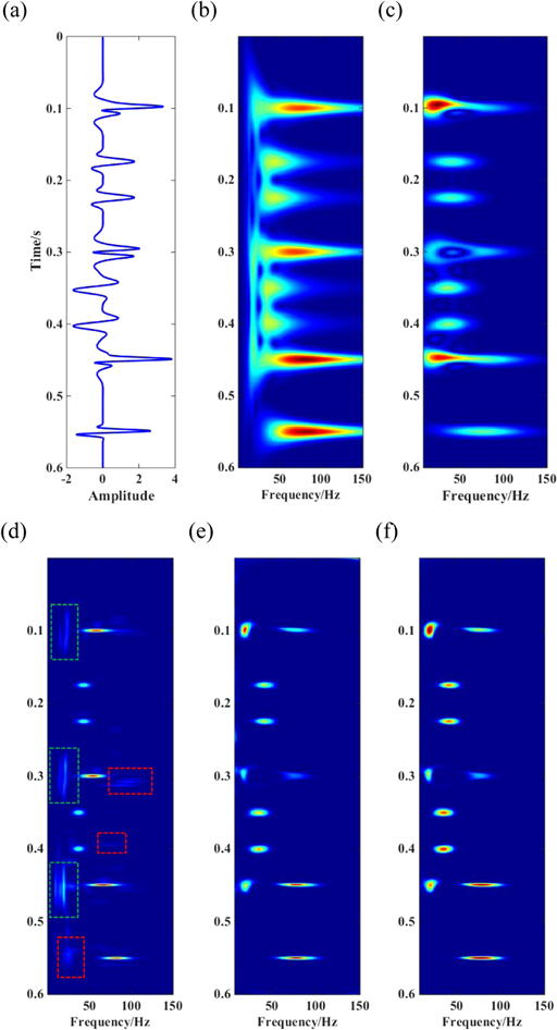
Figure 2. Time-frequency amplitude spectra of a synthetic signal (a), the same as figure 1(a), derived by several spectral decomposition methods, including GST (b), SPWVD (c), MP-WVD (d), IST-IWT (e) and ISD-IST (f).
Download figure:
Standard image High-resolution image(1) In terms of time-frequency resolution, the MP-WVD and ISD, including ISD-IWT and ISD-IST, are vastly superior to the linear transform method GST and the SPWVD. The ISD-IST has a similar advantage as ISD-IWT for resolution. For the mid-and-high frequency components, the MP-WVD has the greatest advantage in time-frequency resolution. However, the results for the low frequency components show unsatisfactory resolution. The green dotted circles in figure 2(d) highlight the results of low frequency with poor resolution. (2) For accuracy, the MP-WVD method is not accurate enough, and is prone to add some interference information or ignore details. Especially when the signal is more complex, the MP-WVD shows more errors. In figure 2(d), red dotted circles point the error locations. Besides, the analysis accuracy of the MP-WVD is limited by the iteration number. An iterative deficiency will result in a wrong conclusion. Along with the MP-WVD, the ISD can provide more accurate results which are in more agreement with the actual information. (3) For computational efficiency, the MP-WVD needs more computing time because of four parameters which need to be calculated in global optimization, i.e. time-shift, amplitude, frequency and phase. The ISD-IWT and ISD-IST have similar calculation time and both of them are more efficient than MP-WVD.
3.1.2. Phase spectra
In seismic exploration, phase information is often associated with important properties such as fluid content and fracturing. Therefore, the study of time-frequency phase information acquisition is an indispensable part of seismic exploration. Generally, due to the influence of time-frequency resolution, conventional spectral decomposition methods place emphasis on the time-frequency amplitude spectrum and ignore the phase spectrum. As a result, most phase information research uses the instantaneous phase attribute. However, the instantaneous phase attribute has many problems, which will be explained later. Thus, extracting phase information is always a difficult problem in signal analysis.
Figure 3(b) is the instantaneous phase spectrum of a synthetic signal, which is displayed in curve and color forms. At the wavelet locations, the phase information of the composite wave can be determined accurately by the instantaneous phase attribute. However, in the locations with no waveform, the values of the instantaneous phase spectrum are not equal to zero, which is obviously unreasonable. Besides, there is another problem: the instantaneous phase spectrum can provide us with the phase information of the composite wave but not the phase details of the different frequency components.

Figure 3. Instantaneous phase (a) and time-frequency phase spectra of a synthetic signal (figure 1(a)) obtained by IST-IWT (b), (c) and ISD-IST (d), (e). Figures show the original phase spectrum (b), (d) and the spectrum with predicted phase details (c), (e).
Download figure:
Standard image High-resolution imageFigures 3(c)–(f) are the phase spectra of ISD-IWT and ISD-IST. Figures 3(c) and (e) are the original phase spectra and 3d and 3f are the spectra with the center time, dominant frequency and predicted phase details. Compared with the instantaneous phase spectrum, the phase spectra from ISD methods make the energy focus into small regions, can provide detailed phase information of the components of composite waves, and make phase values equal to zero in the locations with no waveform. The numerical details in figures 3(d) and (e) show that the predicted phases of both ISD-IWT and ISD-IST are in good agreement with the actual parameters of the wavelet components (shown in figure 1(b)). It is demonstrated that ISD methods are helpful in getting more accurate phase information.
In oil and gas exploration, phase information is very important information for the detection of crack properties and fluid changes. For this, ISD methods may be a good choice.
3.2. Real data
3.2.1. Frequency division
Our real data provided from Hampson-Russell software are recorded over the shallow Cretaceous. The target layer is the gas-bearing sandstone. Figure 4 shows the post-stack seismic profile, the red line is sonic log (the left side corresponds to the small value) and the blue line is the top interface of the gas reservoir. The gas reservoir corresponds to the high-amplitude 'bright spot' at about 0.64 s in the post-stack profile.
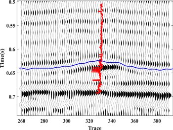
Figure 4. Post-stack profile of a Cretaceous formation. The red line is the sonic log (the left side corresponds to the small value); the blue line is the top interface of the gas reservoir.
Download figure:
Standard image High-resolution imageWe calculated the frequency-division cubes with GST, SPWVD, ISD-IWT and ISD-IST. Figures 5(a), (c), (e) and (g) are the 10 Hz frequency divided sections of the post-stack data by GST, SPWVD, ISD-IWT and ISD-IST methods respectively; figures 5(b), (d), (f) and (h) are the sections at 35 Hz. Figure 5 shows that the result of ISD has not only higher time-resolution but also higher frequency-resolution than GST and SPWVD. When a seismic wave moves through an absorbing hydrocarbon reservoir, attenuation of the high-frequency components is greater than the low-frequency components and this can cause hydrocarbon-induced strong low-frequency energy. As shown in figure 5, ISD (including both ISD-IWT and ISD-IST) with high frequency resolution is helpful in demonstrating the phenomenon of decreasing energy with increasing frequency, and highlighting the gas-bearing area. Besides, compared to GST and SPWVD, ISD with higher time-resolution can better describe the boundary of the gas reservoir. For both time- and frequency resolution, the new ISD-IST method has the same advantage as the traditional ISD-IWT. However, ISD-IST shows us more continuous results with fewer jump-points than ISD-IWT, which demonstrates its higher stability and higher adaptability for real data.

Figure 5. Iso-frequency sections of post-stack data from Hampson-Russell software by using GST (a), (b), SPWVD (c), (d), ISD-IWT (e), (f) and ISD-IST (g), (h) methods for 10 Hz (a), (c), (e), (g) and 35 Hz (b), (d), (f), (h). The red line is sonic log (the left side corresponds to large value); the black line is the top interface of the gas reservoir.
Download figure:
Standard image High-resolution image3.2.2. Phase cube
Through the synthetic signal test in the previous section, we found that it is difficult to obtain phase information with conventional spectral decomposition methods, and ISD methods can get more accurate phase information. Therefore, we calculated the phase cube with the ISD-IWT and ISD-IST methods.
Figures 6(a) and (b) are the phase sections of post-stack data from the Hampson-Russell software, using ISD-IWT and ISD-IST methods respectively. In comparison, both methods can obtain effective phase information from seismic data, and the results have similar resolution. However, the iso-frequency sections of ISD-IST clearly present better stability and lateral continuity than ISD-IWT. From the phase spectrum in figure 6, we find a phase change region which seems to result from the existence of gas, at the location marked by black dotted circles. This demonstrates that the phase spectrum may contain information on the medium and hydrocarbons, and it is suggested that the phase spectrum from ISD methods can be used to extract hydrocarbon information in combination with other detection methods.
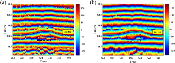
Figure 6. Phase sections of post-stack data from Hampson-Russell software by using ISD-IWT (a) and ISD-IST (b) methods. The black line is the top interface of the gas reservoir; the black dotted circles indicate the phase-change region.
Download figure:
Standard image High-resolution image4. FAVO inversion
Based on the Smith and Gidlow approximation formula, Wilson et al (2009) and Wilson and Adam (2010) expanded the P-wave impedance  and S-wave impedance
  formulae as a Taylor's series and proposed a FAVO inversion formula, written as:
where  is the dominant frequency in a time interval and A and B can be derived in terms of P- and S-velocities and incidence angle. Without considering dispersion, the PP reflection coefficients can be expressed as:

Formula (12) can be written as:

where

 and
and  are the derivatives of impedance with respect to frequency, and we also call them the longitudinal and transverse wave dispersion terms respectively. Using formulae (13), (14) and the convolution formula, we can write the following formula:
Using formula (15), we can use the amplitude spectrum of a wavelet and the time-frequency spectrum of the seismic data to calculate the dispersion term. Generally, hydrocarbons have a strong dispersion effect on longitudinal waves and much smaller effect on transverse waves. Therefore, the longitudinal dispersion term  is more useful in oil and gas detection.
5. Practical application of FAVO based on ISD-IST
The workflow for fluid identification by frequency dependent AVO inversion is as follows: (1) obtain a series of frequency divided cubes based on time-frequency analysis of post-stack data. (2) Analyze the variation characteristics of different frequency sections and determine the fluid-induced frequency anomalies. (3) Using the time-frequency analysis results of pre-stack seismic data and formula (8), calculate the longitudinal dispersion attribute through FAVO inversion. (4) Finally, identify the fluid type by comprehensively analyzing the post-stack frequency anomalies, the well information and the dispersion attributes from FAVO inversion.
We applied the method that combined FAVO inversion with ISD-IWT and ISD-IST to real seismic data from a gas field in Southwest China. The target in our research is a sand-shale interbedded reservoir which has the features of a deep layer, with low permeability and low porosity. Therefore, gas productivity in this research area depends on the fractures. Within the target section, the reservoir sandstones have unequal thicknesses and complex horizontal distributions. Thus conventional methods, including post- and pre-stack inversions and attributes, have difficulty in obtaining satisfactory detection results for gas reservoirs and we try the FAVO method to solve the problem. Figure 7 shows the post-stack seismic profile; the red line is the Gamma well-log curve and the yellow and green curves are the top and bottom interfaces of the target layer. The log-interpretation gas reservoir, indicated by the blue arrow, corresponds to an obviously low Gamma value and the high-amplitude 'bright spot' in the post-stack profile.
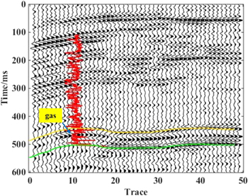
Figure 7. Post-stack profile of an inline survey of a gas field in Southwest China. The red line is the Gamma well-log curve; the yellow and green curves are the top and bottom interfaces of the target layer. The blue arrow indicates the location of the gas reservoir.
Download figure:
Standard image High-resolution image5.1. Gas-induced frequency anomalies from post-stack data
We calculated the frequency-division cubes with SPWVD (which has been often used in FAVO inversion before), ISD-IWT and ISD-IST. Figures 8(a), (c) and (e) are the 10 Hz iso-frequency sections produced by the SPWVD, ISD-IWT and ISD-IST methods respectively; figures 8(b), (d) and (f) are the sections at 25 Hz. The red line in the figures is the Gamma well-log curve and the yellow and green curves are the top and bottom interfaces of the target layer. Because of the absorbing hydrocarbon reservoir, the high-frequency components of the seismic wave usually have stronger attenuation and velocity dispersion than the low-frequency components. This physical mechanism causes the frequency anomaly phenomenon that is characterized by hydrocarbon-induced strong energy at low frequencies and weaker energy for mid-and-high frequencies. This empirical identification helps in recognizing two gas reservoirs, gas 1 and gas 2, by using the frequency-division sections produced by the ISD methods. The predicted gas reservoir 1 is in good agreement with the log interpretation while reservoir 2 is uncertain, and needs further study. The figures undoubtedly demonstrate the better time- and frequency-resolution of the ISD methods and pinpoint the better continuity and stability of ISD-IST compared with ISD-IWT. ISD with good frequency resolution is helpful for demonstrating the seismic low-frequency anomalies and to highlight the gas-bearing area. Besides, compared to ISD-IWT, ISD-IST with better continuity can better describe the boundary of the gas reservoir.
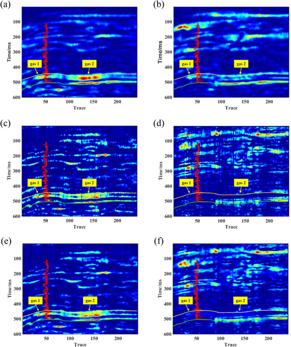
Figure 8. Iso-frequency sections of post-stack data from the gas field in Southwest China produced by using SPWVD (a), (b), ISD-IWT (c), (d) and ISD-IST (e), (f) methods for 10 Hz (a), (c), (e) and 25 Hz (b), (d), (f). The red line is the Gamma well-log curve; the yellow and green curves are the top and bottom interfaces of the target layer.
Download figure:
Standard image High-resolution image5.2. Gas-induced dispersion from pre-stack data
We then calculated the frequency divided cubes of pre-stack angle gathers using SPWVD, ISD-IWT and ISD-IST. FAVO inversion was completed based on the results of frequency decomposition, and longitudinal dispersion sections that correspond to the  term of formula 15 were obtained. Figures 9(a)–(c) shows the partial stack gathers of 1°–10°, 11°–20° and 21°–30° and figures 10(a)–(c) are corresponding time-frequency spectra of the CDP 50 (near the borehore). Figure 11 shows the longitudinal dispersion sections obtained by using SPWVD, ISD-IWT and ISD-ISD respectively. The gas-bearing area is highly attenuative and corresponds to the high dispersion value in the dispersion sections. The gas prediction results from the ISD methods have obviously higher resolution, and are in better agreement with the well information, than SPWVD. Besides, the results obtained from SPWVD cannot describe the reservoir boundary well, because of its lower resolution. The high time-resolution of ISD narrows the predicted gas region, decreases the uncertainty of fluid identification, and provides credible boundary information. Compared to ISD-IWT, ISD-IST shows more continuous results and gives smoother boundary information on the gas reservoir than ISD-IWT. The results demonstrate the higher stability and higher adaptability of ISD for real data.

Figure 9. Profiles of the partial stack data of 1°–10° (a), 11°–20° (b) and 21°–30° (c).
Download figure:
Standard image High-resolution image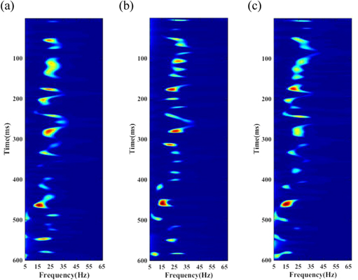
Figure 10. Time-frequency spectra of the CDP 50 of the partial stack gathers using ISD-IST. Figures 10(a)–(c) are the results correspond to 1°–10° (a), 11°–20° (b) and 21°–30° (c) gathers.
Download figure:
Standard image High-resolution image
Figure 11. The longitudinal dispersion sections from FAVO inversion of real data from a gas field in Southwest China based on SPWVD (a), ISD-IWT (b) and ISD-IST (c) time-frequency methods. The red line is the Gamma well-log curve; the yellow and green curves are the top and bottom interfaces of the target layer.
Download figure:
Standard image High-resolution image
By comprehensively analyzing the frequency anomalies (gas-induced frequency anomalies) from post-stack data and the dispersion attributes from FAVO inversion, we have predicted gas reservoirs 1 and 2, which are marked by yellow arrows in figure 11. Gas reservoir 1 has been verified by well information, and reservoir 2 can be proved by drilling results in the future.
6. Conclusions
In seismic exploration, the frequency and phase information of the seismic signal are closely related to the properties of the underground medium. Therefore, the high-resolution spectral decomposition method has become an important tool for property analysis.
In this paper, by comparing the results obtained from the linear transform (GST), bilinear transform (SPWVD and MP-WVD), the traditional ISD (ISD-IWT) and the improved ISD (ISD-IST) methods, we obtain the following conclusions:
- (1)Compared with the GST and SPWVD, the ISD methods (both ISD-IWT and ISD-IST) have higher time- and frequency-resolution. They also have better accuracy and computational efficiency than the MP-WVD.
- (2)The ISD methods not only improve the resolution of the amplitude spectra but also provide more reliable phase spectra. Accurate extraction of the frequency and phase will produce more accurate and comprehensive information for seismic exploration and exploitation.
- (3)For resolution of both amplitude and phase spectra, ISD-IST possesses the same advantages as the traditional ISD-IWT, but has higher stability and higher adaptability than ISD-IWT.
Due to the higher resolution and better accuracy of ISD, we combine FAVO inversion with ISD (including ISD-IWT and ISD-IST) methods. Results from application show:
- (1)High frequency-resolution of ISD is helpful to highlight frequency anomaly phenomena in gas reservoirs and extract gas-induced frequency anomalies from post-stack data.
- (2)The high time-resolution of ISD assists the production of high time-resolution results using FAVO inversion of pre-stack data. The inversion results for gas reservoirs based on ISD are not only in better agreement with well information, but also supply more credible boundary information for the reservoirs. ISD-IST gives more continuous results and smoother boundary information for gas reservoirs than ISD-IWT. All these demonstrate the great advantages and potential of FAVO inversion combined with ISD in hydrocarbon prediction.
Acknowledgments
The authors would like to thank the Associated Editor and anonymous reviewers for their helpful comments, and David Booth for proofreading. This study is sponsored by National Natural Science Foundation of China (grant no. 41574108, 41474096, U1262208) and is to be published with the permission of the EAP sponsors and the Executive Director of the British Geological Survey (NERC).