


Abstract
We report on comprehensive experimental studies of turbulence spreading in edge plasmas. These studies demonstrate the relation of turbulence spreading and entrainment to intermittent convective density fluctuation events or bursts (i.e. blobs and holes). The non-diffusive character of turbulence spreading is thus elucidated. The turbulence spreading velocity (or mean jet velocity) manifests a linear correlation with the skewness of density fluctuations, and increases with the auto-correlation time of density fluctuations. Turbulence spreading by positive density fluctuations is outward, while spreading by negative density fluctuations is inward. The degree of symmetry breaking between outward propagating blobs and inward propagating holes increases with the amplitude of density fluctuations. Thus, blob-hole asymmetry emerges as crucial to turbulence spreading. These results highlight the important role of intermittent convective events in conveying the spreading of turbulence, and constitute a fundamental challenge to existing diffusive models of spreading.
Export citation and abstract BibTeX RIS

Original content from this work may be used under the terms of the Creative Commons Attribution 4.0 license. Any further distribution of this work must maintain attribution to the author(s) and the title of the work, journal citation and DOI.
Edge plasmas are usually strongly turbulent, and manifest intermittency in linear plasma devices and toroidal fusion devices [1–4]. Spreading of turbulence occurs because inhomogeneous turbulence tends to relax and entrain laminar or more weakly turbulent regions [5]. For example, a wake formed downstream of a moving object expands due to the turbulence spreading from the fully turbulent core [6]. Another example is the detection of strong temperature fluctuations inside a magnetic island, due to transient spreading events across it [7]. Generally, turbulence spreading refers to the spatial propagation of turbulence intensity or energy due to nonlinear interactions [5]. Spreading can decouple the intensity field from the local instability growth rate. The observed intensity flux caused by spreading can break Fick's law for the local flux-gradient relation ( ) [8].
Turbulence spreading plays a significant role in the performance of magnetic fusion devices. It is related to the departure of transport scaling from the expected gyro-Bohm scaling [9, 10]. It is important in the core-boundary coupling, and thus affects the H-mode pedestal structure as well as the divertor heat load width [11–15]. Increased turbulence spreading is also associated with the edge cooling approaching density limit and the thermal quench [16–18]. Numerous theoretical [19–29] and simulation [30–36] works have explored the spreading models. But most studies of turbulence spreading are based on a presumed diffusion model, where the turbulence intensity flux is given by the product of diffusivity and intensity gradient, i.e.  . There is a lack of research on the non-diffusive characteristic of turbulence spreading. This is because direct experimental measurements [16, 37–39] of turbulence spreading are still limited.
In this letter, we present comprehensive experimental studies of turbulence spreading dynamics at the tokamak plasma edge. We focus on the non-diffusive characteristics of turbulence spreading and their relation to intermittent convective density fluctuation events (blobs/holes). Turbulence spreading is significantly enhanced at high collisionality or low adiabaticity. Characterizing turbulence spreading as a Fickian diffusion yield an unphysically large or singular diffusivity  , which departs radically from the turbulent particle diffusivity. Turbulence spreading manifests non-diffusive characteristics and thus the usual models are dubious. The turbulence spreading speed (named 'mean jet velocity') correlates linearly with the skewness of density fluctuations. Spreading induced by positive density fluctuation events is outward toward larger radii, and spreading induced by negative density fluctuation events is inward toward smaller radii, as shown by the diagram in figure 1. Increasing symmetry breaking between outgoing blobs and incoming holes causes enhanced turbulence spreading. These results are essential to understand the basic physics of turbulence spreading and to build a foundation for the prediction and interpretation of turbulence transport behaviors.

Figure 1. A simple diagram of turbulence spreading induced by positive (P) and negative (N) density fluctuation events at edge plasma.
Download figure:
Standard image High-resolution imageThe experiments were carried out in Ohmic hydrogen discharges of the J-TEXT tokamak with a limiter configuration [40]. Its major radius and minor radius are  1.05 m and
  0.255 m, respectively. Edge plasmas with different conditions (density, temperature, collisionality and adiabaticity) are obtained by changing the main operation parameters: toroidal magnetic field
  of 1.6–2.2 T, plasma current
  of 125–187 kA and central line-averaged density
  of 2.8–4.9 × 10¹⁹ m−3. The safety factor
  is ∼3.8 in these discharges (shot numbers 1070961–1071002). Collisionality
 ![${\nu ^*} = \left( {{\nu _{ii}}/\varepsilon } \right)/[ {{\varepsilon ^{1/2}}{v_{{\text{th}},i}}/\left( {qR} \right)} ]$](https://content.cld.iop.org/journals/0029-5515/64/6/064002/revision2/nfad40c0ieqn10.gif) and adiabaticity
and adiabaticity  . Here,
  is the ion collision rate,
  is the inverse aspect ratio,
  is the electron thermal speed,
  is the parallel wavenumber,
  is the electron-ion collision rate, and
  is the electron diamagnetic frequency [41]. Since turbulence spreading refers to the spatial propagation of turbulence intensity or energy, it is usually defined as the spatial cross-field flux of turbulence intensity or energy. For turbulence intensity as measured by density fluctuations,
  is the relevant flux. It appears in the evolution equation of turbulence intensity, i.e.
  [34]. For turbulence internal energy,
  is the relevant flux [16]. For turbulence kinetic energy,
  is the relevant flux. Kinetic energy flux is observed to be about two orders of magnitude smaller than internal energy flux in the experiments [15, 16], and so is negligible here. For simplicity, the turbulence spreading flux is calculated as
  . This representation is also widely used in theory and simulations [8, 23].
  at the plasma edge is measured by a Langmuir probe array [16, 37]. Here,
  represents the radial velocity fluctuation and
  stands for the density fluctuation. Electron density
  , temperature
  , plasma potential
  and ion saturation current
  are measured by the triple probe. Ion temperature
  is assumed to be approximately equal to
  . The mean
  poloidal flow
  is calculated as
  . Here,
  indicates a time average. The fluctuating density
  is estimated from ion saturation current fluctuations, i.e.
  . The fluctuating radial velocity
  is inferred from the difference between two poloidally separated floating potential probes, i.e.
  . The sampling rate of probes is 2 MHz. A digital finite impulse response filter is used to obtain the fluctuations with 2
  100 kHz. From the auto-spectra and the wavenumber-frequency spectra of potential fluctuations or density fluctuations, the fluctuations above 100 kHz are at least 2–3 orders of magnitude weaker than those below 100 kHz, and thus are negligible and filtered out.
Figure 2 show the radial profiles of plasma density, electron temperature, electron collision rate  , turbulence spreading flux
  , skewness of density fluctuations and
  poloidal flow velocity, for discharges with different collisionality
  and electron adiabaticity parameter
  near the last closed flux surface (LCFS). Curves with red diamond, green cross, and blue inverted triangle represent edge plasmas with lower
  and higher
  , medium
  and medium
  , higher
  and lower
  , respectively. The black dotted line marks the position of the LCFS at
  = 25.5 cm. We observe that the edge turbulence spreading flux increases as collisionality
  increases or adiabaticity
  decreases, as shown in figure 2(d). For the hydrodynamic regime with
  , density fluctuations
  and potential fluctuations
  are not proportional, as in the adiabatic regime with
  . The electron response thus resembles that of a convective cell [42]. The result shows that as collisions become more frequent and the hydrodynamic response is stronger, edge turbulence spreading grows significantly and becomes more prominent.

Figure 2. The radial profiles of (a) plasma density  , (b) electron temperature
  , (c) collision rate
  , (d) turbulence spreading flux
  , (e) skewness of density fluctuations and (f)
  poloidal flow velocity, for discharges with different collisionality
  and electron adiabaticity parameter
  . (Curves with red diamond correspond to the discharge with
  ,
,  and
and  ; curves with green cross correspond to the discharge with
  ,
,  and
and  ; curves with blue inverted triangle correspond to the discharge with
  ,
,  and
and  ).
).
Download figure:
Standard image High-resolution imageTurbulent diffusion of intensity has long been used as a working model of turbulence spreading. This model has not been tested critically. As the convective properties of edge turbulence increase for higher collisionality in the hydrodynamic regime, the diffusive description of turbulence spreading should be reconsidered. Actually, it has been hypothesized that turbulence kinetic energy spreads via a process independent of turbulent viscosity in the formation of a turbulent wake [6]. The hope that the turbulence energy diffusivity was the same as the turbulent viscosity or particle diffusivity seems unlikely to be realized. Heuristically, we can write:  , where
  is the residual, non-diffusive flux of turbulence intensity. Extracting both
  and
and  from data likely requires dynamics perturbation studies, rather like gas puffing modulation experiments to determine diffusivity
  and convection
  contributions to the particle flux. These would be challenging new experiments, well beyond the scope of this paper. Here, then, we can argue by reductio ad absurdum. So we
- (1)assume

- (2)calculate from the data
- (3)if the calculated measured transport coefficients, then the calculated is likely unphysically large (This is a presumption, of course). So that
- (4), and the residual spreading flux must be retained, i.e. the spreading has a significant non-diffusive component.


The diffusion coefficients of a Fickian model for turbulence spreading flux are calculated and compared to the turbulent particle diffusivity, to test whether the use of diffusive model to describe turbulence spreading is justified or sensible. The turbulence spreading diffusivity is defined as  , while the turbulent particle diffusivity is defined as
  . As illustrated in figure 3, it is obvious that the turbulence spreading diffusivity
  is significantly different from the turbulent particle diffusivity
  . For either the case of lower
  and higher
  (red diamond) or the case of higher
  and lower
  (blue inverted triangle), the profiles of
  vary gently, and are bounded between 0–5
  , as shown in figures 3(c) and (f). However, extremely large turbulence spreading diffusivity
  (10–30
  ) is observed in the region at
  , as shown in figure 3(e). Besides, sharp spikes in the profiles of
  exist in the region at
  , as shown in figures 3(b) and (e). These singular
  values are well over 10
  , up to ∼2000
  . This is because the turbulence spreading flux
  is considerable in these regions, while the local intensity gradient
  is close to zero, as shown in figures 3(a) and (d). The extremely large or spikey unphysical
  in the regions of [
 ] cm clearly highlights the likely non-diffusive component of turbulence spreading (i.e.
  ), and that Fick's law is not sensible for describing turbulence spreading in these regions. It is clear that turbulence spreading is strongly non-diffusive. Besides, when the collisional and hydrodynamic response intensify (i.e.
  goes up and
  goes down),
  increases by ∼2 times, as shown in figures 3(c) and (f), while
  increases by more than 10, as shown in figures 3(b) and (e).
  departs radically from
  . These suggest that the usual diffusive model frequently used to describe the turbulence spreading (with
  ) is invalid.

Figure 3. Turbulence intensity  , turbulence spreading diffusivity
  and turbulence particle diffusivity
  for discharge with lower
  and higher
  (left column, red diamond) and for discharge with higher
  and lower
  (right column, blue inverted triangle). (Curves with red diamond correspond to the discharge with
  ,
,  and
and  ; curves with blue inverted triangle correspond to the discharge with
  ,
,  and
and  .).
.).
Download figure:
Standard image High-resolution imageThe apparently non-diffusive character of turbulence spreading brings to mind the intermittency (bursty events) of density fluctuations due to the presence of coherent structures, such as blobs and holes, within ambient turbulence [43–57]. Thus, we study the relation between turbulence spreading and blobs/holes. Regarding the non-diffusive character of spreading, it is useful to define the mean jet velocity of turbulence spreading  , which can be regarded as the characteristic velocity of spatial propagation of turbulence internal energy [6].
  is effectively an average of radial velocity over the ensemble of density fluctuation intensity. The positive/negative skewness of density fluctuations
  was widely used to identify the existence of blobs/holes, respectively [58]. Figure 4(a) shows the variation of mean jet velocity of turbulence spreading
  versus the skewness of
  in the edge region at
  . There are several measurement data points (typically 3–5) in this region, as shown in figure 2(e). Data points with different symbols correspond to various discharge shot numbers. (
 ,
,  and
and  of Shot No.1070961:
  ,
,  ,
,  ; Shot No.1070962:
  ,
,  ,
,  ; Shot No.1070963:
  ,
,  ,
,  ; Shot No.1070967:
  ,
,  ,
,  ; Shot No.1070980:
  ,
,  ,
,  ; Shot No.1070983:
  ,
,  ,
,  ; Shot No.1070991:
  ,
,  ,
,  .)
.)
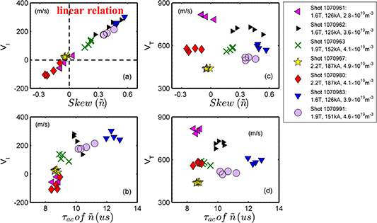
Figure 4. (a) Mean jet velocity of turbulence spreading  VS skewness of density fluctuations
  ; (b) mean jet velocity of turbulence spreading
  VS auto-correlation time of
  ; (c) particle transport velocity
  VS skewness of
  ; and (d) particle transport velocity
  VS auto-correlation time of
  , in the edge region of
  . (Data points with different symbols correspond to various discharge shot numbers.).
Download figure:
Standard image High-resolution imageOur experimental results reveal that the mean jet velocity of turbulence spreading  manifests a linear correlation with the skewness of density fluctuations. As shown in figure 4(a),
  increases linearly with
  .
.  ranges from −100 m s−1 to 300 m s−1 and the skewness ranges from −0.25 to 0.60. It is worth noting that the points of zero skewness and the zero mean jet velocity are approximately coincident. The more positive mean jet velocity of turbulence spreading coincides with the more positive skewness of density fluctuations, while the more negative mean jet velocity coincides with the more negative skewness. This indicates that the positive-dominant density fluctuation events coincide with a radially outward velocity of turbulence spreading, while the negative-dominant density perturbations events coincide with a radially inward velocity of turbulence spreading. The mean jet velocity
  also increases as the auto-correlation time
  of
of  increases, as shown by figure 4(b). Here,
  is determined from the e-folding width of the envelope of the auto correlation function of density fluctuations. The results above demonstrate a strong relation between turbulence spreading dynamics and coherent structures, like blobs and holes.
The particle transport velocity  , which can be seen as the characteristic velocity of turbulent particle transport, has no obvious correlation with both skewness and auto-correlation time, as shown in figures 4(c) and (d). This suggests that the transport of turbulence energy does not simply follow along with turbulent particle transport. Note that the turbulent particle flux is positive (i.e. outward) although the skewness of density fluctuations is negative at
  for the discharge marked with red diamonds in figure 4. Actually, figures 3(c) and 2(e) have shown this result. For all the discharges in our experiments, turbulent particle flux
  and
and  lead to positive (i.e. outward) particle diffusivity
  in the edge region across [
 ] cm. There is no necessary relationship between the sign of skewness of
  and the direction of the particle flux. In contrast to the linear correlation between mean jet velocity
  and
and  , a similar correlation between
  and the kurtosis of
  is not observed.
Figure 5(a) shows the variation of mean jet velocity of turbulence spreading  versus the skewness of
  in the edge region at
  . It shows results consistent with those shown in figure 4. The mean jet velocity
  exhibits a linear correlation with the skewness of
  . The more positive mean jet velocity
  coincides with the more positive skewness of
  .
.  increases as
  of
of  increases. These results again demonstrate a strong relation between turbulence spreading dynamics and coherent structures, like blobs and holes. Note that the negative (i.e. inward) mean jet velocity of turbulence spreading is not observed in this region of
  . As shown by figure 2(e), the skewness of density fluctuations is positive in this region. We should point out that in another edge region of
  , the mean jet velocity of turbulence spreading
  has no obvious correlation with
  skewness and auto-correlation time. This may be due to the existence of edge
  poloidal flow shear in this region, as shown by figure 2(f). A strong
  shear layer exists in the region of
  [
[ ] cm, while the
  flow shear is rather weak in the region of
  [
[ ]
]  and
and  [
[ ] cm. The sheared flow might cause the decorrelation, distortion and breaking of turbulence eddies and blob/hole structures [59–61], resulting in the breakdown of relation between turbulence spreading velocity and skewness/auto-correlation of density fluctuation events. The interactions between blob dynamics and sheared flow are interesting, but are out of the scope of this letter, which emphasizes the non-diffusive character of turbulence spreading. Here, we focus on the regions of [
 ] cm of unphysically large or singular spreading diffusivity
  , where the turbulence spreading flux
  is considerably large but the intensity profile is rather flat, as shown by figure 3(d).

Figure 5. (a) Mean jet velocity of turbulence spreading  VS skewness of density fluctuations
  ; (b) mean jet velocity of turbulence spreading
  VS auto-correlation time of
  ; (c) particle transport velocity
  VS skewness of
  ; and (d) particle transport velocity
  VS auto-correlation time of
  , in the edge region of
  . (Data points with different symbols correspond to various discharge shot numbers.).
Download figure:
Standard image High-resolution imageNote that skewness measures the asymmetry of probability distribution function. The strong correlation between mean jet velocity and skewness suggests the importance of blob-hole asymmetry to turbulence spreading. Figure 6(a) shows the distribution of turbulence spreading flux as a function of density fluctuation amplitude in the region of spikey, unphysical spreading diffusivity  at
at  . The horizontal coordinate is the density fluctuation amplitude normalized to a multiple of the standard deviation, i.e.
  . The vertical coordinate is the accumulated and averaged turbulence spreading contributed by the density fluctuations within a certain range of amplitude, i.e.
 ![${P_{{\text{spreading}}}}\left( A \right) = [ {\mathop \sum \nolimits_{\left( {A - 0.05} \right){\sigma _{\tilde n}} \lt \tilde n \lt \left( {A + 0.05} \right){\sigma _{\tilde n}}} ({{\tilde v}_{\text{r}}}{{\tilde n}^2}/2)} ]/M$](https://content.cld.iop.org/journals/0029-5515/64/6/064002/revision2/nfad40c0ieqn232.gif) for positive
for positive  and
and ![${P_{{\text{spreading}}}}\left( A \right) = [ {\mathop \sum \nolimits_{ - \left( {A + 0.05} \right){\sigma _{\tilde n}} \lt \tilde n \lt - \left( {A - 0.05} \right){\sigma _{\tilde n}}} ({{\tilde v}_{\text{r}}}{{\tilde n}^2}/2)} ]/M$](https://content.cld.iop.org/journals/0029-5515/64/6/064002/revision2/nfad40c0ieqn234.gif) for negative
for negative  . The radial velocity fluctuations with the same temporal sampling interval corresponding to the
  amplitude range are taken for the calculations.
  , which is the total number of sampling points of
  or
or  . The total turbulence spreading flux is the sum of distribution function, i.e.
  .
.
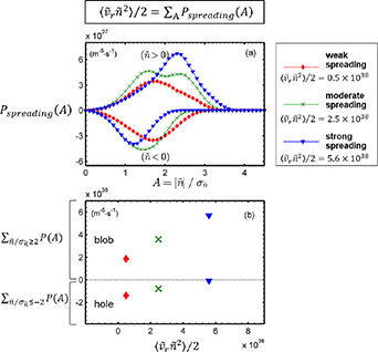
Figure 6. (a) The distribution of turbulence spreading flux  relative to the density fluctuation amplitude
  ; (b) the contribution of blob with
  and hole with
  to the total turbulence spreading
  , in the edge region of
  .
.
Download figure:
Standard image High-resolution imageFigure 6(a) shows that, the turbulence spreading flux induced by positive density fluctuations is positive, i.e. the turbulence intensity contributed by positive  propagates outward. The turbulence spreading flux induced by negative density fluctuations is negative, i.e. the turbulence intensity contributed by negative
  propagates inward. The net total turbulence spreading flux
  is obtained from the sum of positive and negative components, as given by the values in the legend of figure 6(a). Note that for the case of weak spreading, marked by red diamonds, the distribution function is nearly symmetric. For increasing outward spreading, marked by green crosses and blue inverted triangles, the distribution function is strongly asymmetric. The positive contribution of high-amplitude positive density fluctuations increases while the negative contribution of high-amplitude negative density fluctuations decreases. This is especially true for the contribution of blobs and holes with absolute amplitudes higher than
  . This can be directly seen from figure 6(b). The blobs-dominant events with
  cause radially outward turbulence spreading, while the holes-dominant events with
  cause a radially inward turbulence spreading. For increasing total turbulence spreading
  , the positive components contributed by blobs, i.e.
  increase, while the negative components contributed by holes, i.e.
  decrease. The increased symmetry breaking between positive and negative density fluctuation—i.e. blob-hole asymmetry—events causes enhanced net turbulence spreading. These results explain the previous observation of the correlation between the mean jet velocity of spreading and the skewness of density fluctuations in figure 5(a).
Figure 7(a) shows the distribution of turbulence spreading flux  as a function of density fluctuation amplitude
  in the region of extremely large turbulence spreading diffusivity
  at
at  , as shown in figure 3(e). It also shows that the turbulence spreading flux induced by positive density fluctuations is positive, and the turbulence spreading flux induced by negative density fluctuations is negative. For enhanced outward spreading, marked by green crosses and blue inverted triangles, the distribution function is more asymmetric. This is especially true for the contribution of blobs and holes with absolute amplitudes higher than
  . It is noted that for the increased outward spreading, the contribution of blobs (
 ) to spreading even decreases slightly, as shown by the green crosses and blue inverted triangles in figure 7(b). The enhanced net total outward spreading is not related to the increased contribution of blobs (
 ) but the decreased contribution of holes (
 ) in this region. The increased symmetry breaking between positive and negative density fluctuation events—with
  dominant—causes enhanced outward turbulence spreading. We also note that the symmetry breaking between positive and negative density fluctuation events—with
  dominant—causes the total net inward turbulence spreading, as shown by the red diamond symbol. Recall that the negative (or inward) turbulence spreading flux in the region at
  for the case with lower
  and higher
  shown by figure 2(d), and that the inward mean jet velocity of spreading coincides with the negative skewness of density fluctuations shown by figure 4(a).

Figure 7. (a) The distribution of turbulence spreading flux  relative to the density fluctuation amplitude
  ; (b) the contribution of blob with
  and hole with
  to the total turbulence spreading
  , in the edge region of
  .
.
Download figure:
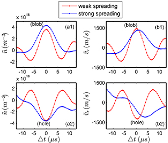
Standard image High-resolution imageTo further explore the role of blob-hole dynamics in turbulence spreading, conditional average [47, 62] methods, which are routinely used to isolate blobs and holes from ambient turbulence, are adopted in our work. The conditional average results of  in the region of spikey, unphysical spreading diffusivity
  at
at  for discharges with weak and strong turbulence spreading are shown in figures 8(a1) and (a2). The time window of counting blobs and holes is
  corresponding to 6000 sampling points. The conditional average curve is obtained by averaging the accumulation of burst events with a peak value exceeding the threshold of
  in a time interval of
  around the peak. The time coordinates of burst events in
  are used to select the time series of
  . The conditional average results of
  are shown in figures 8(b1) and (b2). The temporal and spatial features of blobs and holes can be obtained by analyzing the conditional average results. The burst rate
  of blobs and holes, which is the number of burst events in
  divided by the total time they are counted, characterizes the intermittency of density fluctuations. The life time
  of blobs and holes is determined from the full width at 1/e of the peak value in the conditional average of
  . The radial propagation speed
  of blobs and holes is estimated from the mean value of conditional averaged
  during the life time. The characteristic radial length of blobs/holes are calculated by the product of the life time and the radial propagation speed, i.e.
  .
.
Figure 8. Conditional average results of  and
and  for discharges with weak turbulence spreading and strong turbulence spreading.
Download figure:
Standard image High-resolution image
The burst rate  , life time
  , radial propagation speed
  and characteristic radial length
  of blobs and holes for weak/strong turbulence spreading are given in table 1. We also give the values of some familiar relevant quantities to facilitate the appreciation of the temporal and spatial features of blobs/holes. As turbulence spreading becomes stronger: (i) the burst rate of blobs increases from ∼7.9 kHz to ∼12 kHz, while the burst rate of holes decreases prominently from ∼9.1 kHz to ∼0.3 kHz. Here, the electron diamagnetic drift frequency
  is ∼45 kHz for weak spreading and ∼12 kHz for strong spreading. (ii) the life time
  of blobs and holes increases simultaneously from ∼8
  to ∼10
  , which is reasonable since
  of
of  is ∼9
is ∼9  for weak spreading and ∼14 μs for strong spreading. (iii) the radial propagation speed
  of blobs increases from 70 m s−1 to 630 m s−1 and
  of holes increases from −18 m s−1 to −360 m s−1. Here, the mean jet velocity of turbulence spreading
  increases from ∼55 m s−1 to ∼350 m s−1, while the electron diamagnetic drift velocity
  decreases from ∼1550 m s−1 to ∼570 m s−1. Note that the mean jet velocity is somewhere between the radial propagation speed of blobs and holes, for either weak spreading or strong spreading. This outcome is reasonable, as the mean jet velocity is an ensemble averaged quantity. (iv) the characteristic radial length
  of blobs increases (from 0.6 mm to 6.6 mm) and
  of holes also increases (from 0.1 mm to 3.7 mm). For weak spreading, the characteristic radial lengths
  of blobs and holes are close to the ion gyro radius
  ∼ 0.3 mm. For strong spreading,
  of blobs and holes are close to the radial correlation length of density fluctuations
  ∼ 4.4 mm. This is reasonable as figure 8 implies that regimes of strong spreading are necessarily blob dominated.
Table 1. The burst rate, life time, radial propagation speed and characteristic radial length of blobs/holes for weak/strong turbulence spreading.
| Turbulence spreading case | Spreading flux  ( ( ) ) | Burst rate  (
( ) )
| Life time  (μs)
(μs)
| Propagation speed  (m s−1)
| Characteristic radial length  (mm) (mm) | ||||
|---|---|---|---|---|---|---|---|---|---|
| Blobs | Holes | Blobs | Holes | Blobs | Holes | Blobs | Holes | ||
| Weak | 0.5 × 1038 | 7.9 | 9.1 | 8.1 | 8.2 | 70 | −18 | 0.6 | 0.1 |
| Strong | 5.6 × 1038 | 12 | 0.3 | 11 | 10 | 630 | −360 | 6.6 | 3.7 |
Note that  of blobs are positive and
  of holes are negative, indicating blobs move outward while holes move inward. This is consistent with previous studies [58]. This again shows that positive density fluctuation events cause radially outward spreading of turbulence intensity (
 ), while negative density fluctuation events cause radially inward spreading of turbulence intensity (
 ), as presented in figure 8. For the case with weak turbulence spreading, the burst rate of blobs and holes are very close to one another, which corresponds to the nearly symmetrical distribution function of spreading flux in figure 6(a). For the case with strong turbulence spreading (where the collisionality
  is high and adiabaticity
  is low), the burst rate of blobs is about 40 times larger than that of holes, which corresponds to a remarkable symmetry breaking in the distribution function of the spreading flux. Therefore, the difference in burst rates of blobs and holes plays a significant role in the turbulence spreading dynamics. For strong spreading, the width of the singular turbulence spreading diffusivity (
 ) region with
  is ∼5 mm, shown by figures 3(d) and (e). This width falls between the characteristic radial lengths
  of blobs and holes, i.e. 3.7–6.6 mm. This clarifies the importance of intermittent convective coherent events to turbulence spreading.
To summarize, an in-depth study of turbulence spreading and its relation to convective coherent structures was carried out by using direct experimental measurements of edge plasmas. Results indicate that turbulence spreading is significantly enhanced as collisions become more frequent and the electron response becomes hydrodynamic. Turbulence spreading is shown to be strongly non-diffusive. Attempts to characterize turbulence spreading as a Fickian diffusion process yield a singular (spikey, unphysical) profile of turbulence spreading diffusivity  , which departs significantly from the turbulent particle diffusivity
  . Thus, turbulence spreading is not amenable to characterization as a diffusion process with a diffusivity closely related to the turbulent diffusivity, as often assumed. To quantify the strength of spreading, it is useful to define the mean jet velocity of turbulence spreading
  . The mean jet velocity
  manifests a linear correlation with the skewness of density fluctuations. The zero point of skewness and the zero point of the mean jet velocity approximately intersect. The more positive mean jet velocity of turbulence spreading coincides with the more positive skewness of density fluctuations, while the more negative mean jet velocity coincides with the more negative skewness.
  increases with the auto-correlation time of
  while the particle transport velocity
  does not. This suggests that the transport of turbulent internal energy does not simply follow along with turbulent particle transport. The distribution of turbulence spreading flux exhibits interesting trends in its dependence on amplitudes of positive density fluctuations and negative density fluctuations. Turbulence spreading flux induced by positive density fluctuations is positive, i.e. propagating outward. Turbulence spreading flux induced by negative density fluctuations is negative, i.e. propagating inward. For the case with weak turbulence spreading, the burst rate of blobs and holes are very close to each other and the distribution function is symmetrical. For the case with strong turbulence spreading at higher collisionality or lower adiabaticity, the burst rate of blobs is much larger than that of holes and the distribution function of spreading flux is strongly asymmetric. The increased symmetry breaking between convective coherent structures, i.e. asymmetry between the populations of outgoing blobs and incoming holes, causes enhanced net spreading. The width of the region with singular turbulence spreading diffusivity (
 ) and
) and  falls between the characteristic radial lengths of blobs and holes. These results clarify the importance of intermittent convective coherent events in the basic structure of turbulence spreading. Spreading is seen to be fundamentally intermittent and non-diffusive. These results present a significant challenge to conventional models of turbulence spreading.
Regarding future work, we note that recently, there has been a resurgence of interest in turbulence spreading and related phenomena in the context of SOL heat load width or power scrape off width ( ) broadening. In many cases, especially in H-mode conditions, local SOL turbulence is quenched, so
  collapses to the neoclassical prediction, which is unacceptably small. The hope is that turbulence spreading from the pedestal may sufficiently energize SOL turbulence, so as to broaden
  with enhanced cross-field transport [13]. More generally, some recent studies indicates that even in L-mode, spreading from the edge has a significant or even dominant impact on SOL turbulence levels, and thus on the SOL width. The findings of this letter indicate that such edge
  SOL spreading is strongly intermittent and carried by structures (blobs). Thus, mean field models are destined to fail. The natural characteristic velocity for this spreading process is the jet or spreading velocity
  . Figure 4(a) shows that
  correlates well with the skewness (indicative of structures) and with spreading. Thus, we conjecture that the SOL width resulting from spreading-induced broadening is
  . Here,
  is the SOL dwell time constrained by either the heat residence time or the auto-correlation time of turbulence, whichever is shorter. The detailed dependence of the heat residence time varies with collisionality. The relevant comparison is then
  vs
vs  , where
  , and
, and  is the magnetic drift velocity. In this case,
  . Thus, the natural figure of merit for comparing spreading and neoclassical processes is based on comparison of jet and drift velocities, i.e.
  and
and  . This should be contrasted to the conventional approach, which is to compare
  to
to  . In particular, the conventional wisdom does not account for the coherence and cross phase of
  with
with  . This cross phase encapsulates the key physics of spreading. Similarly, criteria tied to turbulent transport are necessarily based upon the transport cross phase in
  . This differs fundamentally from that which appears in
  . In another word, turbulence spreading flux depends upon the coherence and cross phase of
  with
with  , while the turbulent particle flux depends upon the coherence and cross phase of
  with
with  . Increasing
  will likely be beneficial to increase spreading flux and particle flux, but the actual spreading flux and particle flux need not increase in direct proportion, or even in the same direction simultaneously. Inward turbulence spreading but outward particle transport in the region of
  has been observed for the discharge marked by red diamonds in figure 4 (also figures 2 and 3). Future work will focus on testing the conjecture set forth above and on quantifying the parametric dependences of the jet velocity.
We should also point out that, in our experiments, the collisionality near the LCFS is higher than 1 and the adiabaticity near the LCFS is lower than 1 (corresponding to the hydrodynamic regime). However, collisional plasmas are not always hydrodynamic. Theoretically, while the plasma edge is usually collisional, it can be either adiabatic or hydrodynamic, depending upon  . Turbulence in the adiabatic regime is observed to support avalanches. Turbulence avalanching involves turbulence spreading. Avalanches manifest 'bumps' (i.e. local excesses) or 'holes' (i.e. local deficits) in simulation works [8]. A further comment is given in the
Acknowledgments
P. H. Diamond, Rongjie Hong and Mingyun Cao thank Filipp Khabanov, Zheng Yan, George Tynan and George Mckee for stimulating discussions of a related ongoing project. This work is supported by: the Ministry of Science and Technology of the People's Republic of China under Grant No. 2022YFE03100004; the National Natural Science Foundation of China under Grant Nos. 51821005 and 12375210; the Science and Technology Department of Sichuan Province under No. 2022JDRC0014; the Chengdu Science and Technology Project under 2022TFQCCXTD. The work is also supported by the U.S. Department of Energy, Office of Science, Office of Fusion Energy Sciences under Award Number DE-FG02-04ER54738 and the Sci DAC ABOUND Project, scw1832. The authors would like to thank the Isaac Newton Institute for Mathematical Sciences, Cambridge, for support and hospitality during the programme [Anti-diffusive dynamics: from sub-cellular to astrophysical scales (ADI)] where work on this paper was discussed. This work was supported by EPSRC Grant No EP/R014604/1.
Appendix:
One can distinguish two types of classification regarding the regimes for electron response: (i) collisional vs collisionless—determined by collision mean free path vs connection length, i.e. 

 vs
vs 

 , where
  and
and  ; (ii) hydrodynamic vs adiabatic—depending upon
 vs
vs  . In practice, here
  is used and all other quantities are measured. The adiabatic regime has electrons responding along the magnetic field at a rate exceeding the wave frequency). Then,
  and the fluctuations are drift wave like. The hydrodynamic regime is one of convective cells, where electrons oscillate faster than their response along the magnetic field. The collisionless electron response (

 ) is almost always adiabatic (
 ) unless
  . While the plasma edge is usually collisional, it can be either adiabatic or hydrodynamic, depending upon
  . In a burning plasma, the edge is more likely (but not definitely) to be adiabatic. Turbulence spreading can surely persist in adiabatic electron regimes. For wavelike fluctuations, a piece of turbulence spreading is simply the wave energy density flux [63], i.e.
  . Here,
  is the wave energy density and
  is the radial group velocity. This coexists with the eddy mixing process with
  . The ratio of these two is closely related to the Kubo number, i.e.
  . Turbulence spreading of wave energy can be alive and well in the adiabatic regime, when
  is small. There are numerous gyrokinetic simulations which study turbulence spreading in collisionless or nearly collisionless regimes with adiabatic electrons. These are summarized in the paper by T.S. Hahm and P.H. Diamond [8]. Simulation results show that turbulence spreading in the collisionless regime is closely related to avalanches. These avalanches manifest 'bumps' (i.e. local excesses) or 'holes' (i.e. local deficits), somewhat akin to 'blobs' and 'holes'. A precise comparison and contrast between these two sets of classification has not yet been undertaken. Whether the turbulence spreading in the adiabatic regime is related to the dynamics of 'blobs and holes' is still unresolved.