


Abstract
Kinetic equilibrium reconstruction plays a vital role in the physical analysis of plasma stability and control in fusion tokamaks. However, the traditional approach is subjective and prone to human biases. To address this, the consistent automatic kinetic equilibrium reconstruction (CAKE) method was introduced, providing objective results. Nonetheless, its offline nature limits its application in real-time plasma control systems (PCSs). To address this limitation, we present RTCAKENN, a machine learning model that approximates 7 CAKE-level output profiles, namely pressure, inverse q, toroidal current density, electron temperature and density, carbon ion impurity temperature and rotation profiles, using real-time available inputs. The deep neural network consists of an encoder layer, where the scalars and interdependent inputs such as plasma boundary coordinates and motional Stark effect data are encoded using multi-layer perceptrons (MLPs), while profile inputs are encoded by 1D convolutional layers. The encoded data is passed through a MLP for latent feature extraction, before being decoded in the decoding layers, which consist of upsampling and convolutional layers. RTCAKENN has been implemented in the DIII-D PCS and our model achieves accuracy comparable to CAKE and surpasses existing real-time alternatives. Through clever dropout training, RTCAKENN exhibits robustness and can operate even in the absence of Thomson scattering data or charge exchange recombination data. It executes in under 8 ms in the real-time environment, enabling future application in real-time control and analysis.
1. Introduction
One crucial aspect in the physical analysis of plasma stability and transport in tokamaks involves the reconstruction of magneto-hydrodynamic (MHD) equilibria [1, 2], for instance, through methods like EFIT [1]. Not only the internal plasma pressure and magnetic field structure but also magnetic flux coordinates can be provided for detailed physics calculations through MHD equilibrium reconstruction. In particular, accurate plasma equilibria are required for 3D MHD stability analyses, such as JOREK [3], DCON [4] and STRIDE [5]. When only magnetics are included, the plasma shape can be robustly and accurately reconstructed, while internal plasma profiles remain unconstrained. Recently, many tokamaks have been reconstructing more accurate kinetic equilibria based on various diagnostic signals, such as motional Stark effect (MSE) [6, 7], Thomson scattering (TS) [8], charge exchange recombination (CER) spectroscopy [9], and high-fidelity physical calculations, such as NUBEAM [10] (a Monte Carlo package for evaluation of the deposition, slowing down, and thermalization of fast ion species in tokamaks) and NEO [11] (a multi-species drift-kinetic solver tool for high accuracy neoclassical calculations), to constrain the internal plasma information. However, the fitting process from noisy multiple diagnostic signals can be affected by researchers' subjectivity, and a considerable amount of iterative computation with NUBEAM and EFIT is required, resulting in high-cost time consumption for researchers. Therefore, the Consistent Automatic Kinetic Equilibria (CAKE) workflow has been developed to minimize researchers' subjectivity during the process and perform efficient kinetic equilibrium computations for many discharges [12]. This enables statistical stability analysis for various discharges and provides initial input for manual fine-tuning of kinetic equilibria. Furthermore, it demonstrated the concept of fully automated reconstruction that can be applied to plasma prediction and control. Recently, studies on real-time plasma profile prediction [13], control [14, 15] and profile-based instability avoidance [16] have been initiated. Real-time capable kinetic equilibrium reconstruction technology will further advance plasma profile-based prediction and control. However, the current CAKE workflow still requires a large amount of iteration with NUBEAM, NEO, and EFIT computations, which take at least several minutes if not hours per each time slice, limiting its application for real-time control.
Recently, machine learning (ML)-based acceleration techniques have been applied to various tokamak physics calculations [17, 18]. With ML, it is possible to quickly generate kinetic equilibria through an end-to-end approach from various plasma diagnostic signals. This study aims to develop a fast kinetic equilibrium reconstruction tool suitable for real-time prediction and control, by training ML models with kinetic equilibrium data for tens of thousands of time slices reconstructed through the CAKE workflow. The remainder of this paper is as follows. In section 2 we discuss input selection, the ML model architecture and training. The implementation of RTCAKENN in the DIII-D plasma control system (PCS) is presented in section 3, followed by experimental demonstrations in section 4 where we highlight model accuracy, robustness and timing.
2. ML modeling: RTCAKENN
The input information that kinetic equilibrium reconstruction requires can be divided into four categories based on their dimensions and interdependence. The first category includes scalar independent variables, such as toroidal magnetic field strength and plasma current. Second, there are scalar interdependent variables, the pitch angles of the internal magnetic field lines measured by MSE. The third one consists of one-dimensional signals of plasma pressure and current density (or safety factor, q) profiles obtained from real-time EFIT used as initial conditions, as well as electron density, electron temperature, ion temperature, and ion rotation frequency profiles measured through TS and CER. Here, the toroidal ion rotation frequency (Ωtor) refers to the angular frequency (Ωtor = 2πftor), where ftor is the general rotation frequency in Hz. Lastly, two-dimensional coordinate information of the plasma boundary obtained through magnetic measurements and real-time EFIT is also necessary (throughout this work real-time EFIT refers to the version that only relies on magnetics, no kinetic data). These pieces of information have different dimensions, and even within the same dimension, they have different spatial resolutions depending on the diagnostic system used. The output signals calculated from this multimodal information are the profiles of plasma pressure, safety factor, current density, electron density, electron temperature, ion temperature, and ion rotation velocity, which satisfy the kinetic MHD equilibrium. Here, we decided not to include higher-dimensional information such as 2D magnetic flux surfaces in the output. This omission was not due to any incapability but rather was a strategic choice to avoid computational time delays, especially considering that it is of lesser significance from the control perspective, the primary aim of real-time analysis. Moreover, it is worth noting that this 2D flux surface information is inherently embedded in the remaining outputs, and during offline analysis, it can be mapped one-to-one using the Grad–Shafranov equation. Note that throughout this paper, whenever we refer to j or the current density profile, the flux surface averaged toroidal current density is meant. Additionally, in the CAKE code, all 'ion' quantities actually represent the C6+ ions. The carbon impurity temperature is employed as an analogue to the bulk temperature. It is important to note that while this approximation serves well for the central region, it may not accurately represent the ion temperature at the plasma edge. To mitigate this limitation, CAKE excludes edge measurements of C6+ temperature and instead utilizes an assumption of (bulk ion temperature to electron temperature) ratio 'stiffness' to extrapolate the bulk ion temperature in the edge region. This extrapolation ensures a more comprehensive representation of ion temperatures throughout the plasma. Similarly, the rotation profile fit is determined based on impurity ion data as well. More detailed information about the inputs and outputs can be found in table 1. In this study, the deep neural network architecture depicted in figure 1 is used to generate the desired output information by taking in multiple inputs of different dimensions.


Figure 1. Neural network architecture for multimodal prediction of kinetic equilibrium profiles.
Download figure:
Standard image High-resolution imageTable 1. Input and output signals for the multimodal neural network.
| Inputs | Description | Source | Mean/Std |
|---|---|---|---|
| Bt | Toroidal magnetic field strength (T) | Magnetics | 0.242/1.95 |
| Ip | Plasma current (A) | Magnetics | (1.04/0.280) × 106 |
| γi | Magnetic field pitch angles i | MSE | 0.104/7.29 |
| (R, Z) | R and Z of plasma boundary (m) | RT-EFIT | (1.55/0.414, −0.0314/0.707) |
| p | Pressure profile (Pa) | RT-EFIT | (2.69/2.37) × 104 |
| q | Safety factor profile | RT-EFIT | 2.78/2.34 |
| ne | Electron density profile (1019 m−3) | TS | 4.06/1.86 |
| Te | Electron temperature profile (keV) | TS | 1.52/1.02 |
| Ti | Ion temperature profile (keV) | CER | 1.66/1.11 |
| Ωtor | Toroidal rotation frequency (kHz) | CER | 38.1/28.3 |
| Outputs | Description | True result | Mean/Std |
| p | Pressure profile (kPa) | CAKE | 22.3/22.4 |
| j | Current density profile (MA m−2) | CAKE | 0.642/0.660 |
| q | Safety factor profile | CAKE | 1.01/5.18 |
| ne | Electron density profile (1019 m−3) | CAKE | 3.72/1.96 |
| Te | Electron temperature profile (keV) | CAKE | 1.31/1.02 |
| Ti | Ion temperature profile (keV) | CAKE | 1.49/1.23 |
| Vtor | Toroidal rotation velocity (km s−1) | CAKE | 67.6/52.6 |
The signals diagnosed in a tokamak have different dimensions and resolutions, and it is necessary to map these signals to consistent sets of coordinates for input feeding into a neural network, as shown in figure 1(a). To do this, several preprocessing steps are required to obtain the input signals during model training and inference. First, RT-EFIT calculations are required for the plasma boundary coordinates and MHD pressure and safety factor profiles in the input signals. Note that the results from RT-EFIT are also used as the initial guess state for iterations in manual kinetic equilibrium reconstruction. In this study, the resolution (N in figure 1(a)) of the plasma boundary coordinates estimated by RT-EFIT was set to N= 8. Therefore, eight (R, Z) coordinate values at the innermost, outermost, top, bottom, and middle-index points were used as input. Additionally, RT-EFIT provides the poloidal magnetic flux, ψN , which is the domain coordinate for 1D input signals. Subsequently, the kinetic profiles diagnosed through TS and CER are mapped to this ψN coordinate during the preprocessing step.
Then, the preprocessed input signals are fed into the neural network model, as shown in figure 1(b). First, the magnetic pitch angles diagnosed by MSE are interdependent scalar values, and they are encoded by a multi-layer perceptron (MLP) in the model. The 2D plasma boundary (R, Z) coordinates, which are also composed of interdependent values, are encoded by another MLP. The kinetic profile signals of plasmas are 1D information mapped to the magnetic flux coordinate, ψN. Considering their dimensional characteristics, they are encoded by 1D convolutional layers for effective feature extraction. The signals of magnetic field strength and plasma current are already small-size independent variables, so they are concatenated with other encoded information without additional encoding.
After the encoding process, the comprehensive latent features are extracted from the concatenated information of encoded signals by MLP (figure 1(c)). Lastly, from these latent features, the final kinetic profiles that satisfy the MHD equilibrium are generated by decoder networks shown in figure 1(d) comprising upsampling and convolutional layers. The final output profiles are composed of seven 1D features described in table 1. The detailed description of the neural network architecture is shown in
For training the neural network, we used the kinetic equilibria reconstructed via CAKE [12], which are stored in the OMFIT database [19]. The dataset contains a total of 696 discharges at 18 959 time points. The dataset did not get biased or focused on specific scenarios and as such includes L-mode and H-mode plasmas as well as instances with ITB or hybrid-like scenarios. CAKE can occasionally generate outlier results due to low-quality diagnostics. Therefore, we filtered out excessive outliers that are not in the typical operating region of DIII-D. Filtering out outliers is an automated process that involves excluding cases that surpass pre-specified limits, and this is carried out before the model's training. The mean and standard deviation values for the filtered dataset are listed in table 1. Here, the toroidal magnetic field (Bt ) in inputs, and the current density (j) and safety factor (q) in outputs are signed quantities according to their direction, which leads to the mean values being smaller than the standard deviation values. Additionally, as the safety factor q can diverge to infinity at the boundary of diverted plasma, we utilized the inverse of the safety factor, 1/q, for numerical convenience. We used Adam [20] as the optimizer and set the loss function to mean squared error for optimizing the model. To reduce the risk of overfitting, we implemented the early-stopping method, which relies on the validation loss. Additionally, we created an ensemble model by employing ten different models with identical architectures [21]. By using this approach, the outputs of each internal model are averaged, leading to smoother profiles and the algorithm becomes more robust against outliers from individual models. The training of these models was performed using the Keras API [22], and the trained Keras model was converted to C code using the Keras2C library [23] for implementation on DIII-D PCS.
In actual tokamak experiments, there are often cases where TS and CER diagnostics are not available or have low reliability for various reasons. Employing imprecise diagnostics or estimated profiles to reconstruct kinetic equilibria may result in unrealistic and inconsistent outcomes. One of the goals of this study is to obtain reliable kinetic equilibrium even in the absence of some diagnostic signals. To achieve this, during the input feeding process when training the model in figure 1(a), we employed a dropout technique on TS or CER input data with a rate of 0.1. For this dropout, the input data is set to zeros or randomly determined within the normal operation range with a half-and-half probability. This way enables the model not to overly rely on the TS and CER inputs when estimating the final kinetic equilibrium. With this approach, the trained model can infer missing signals from the remaining signals when TS or CER signals are absent or unreliable in actual tokamak experiments. This inherently assumes that the different profiles are sufficiently interdependent, allowing for the estimation of missing information based on the available information. For example, in the absence of TS diagnostics, we may not have direct inputs for electron density and electron temperature, but we can provide ion temperature, pressure profiles, and q profiles. The pressure and ion temperature can offer indirect information on the possible ranges of electron density and temperature, and also allow us to estimate the electron temperature gradient regulated by ion temperature gradient turbulence. The q profiles and rotation profiles also provide additional support for electron confinement. Similarly, in the absence of CER, indirect information can be provided in the reverse direction. While the profiles estimated from the remaining inputs may have differences from actual profiles, it is a reasonable approach to estimate equilibrium profiles when some diagnostic data is unavailable during actual operation. The input dropout technique also helps prevent the overfitting of the model. Additionally, by keeping the input dropout rate low (0.1), we intended to allow for the utilization of actual input signals when they are available.
Figure 2 presents regression plots of the output variables computed using the trained model (upper) and distributions of the corresponding errors (lower). The test data shown in figure 2 are composed of 1334 time-slices and have not been used in training. Note that during this test regression, the input dropout was not applied. Panels (a)–(g) represent the output variables listed in table 1. The Pearson R metrics, serving as indicators of accuracy between the true and predicted values, are also displayed on the regression plots. The average value of R across the seven profile predictions is 0.972, and even the lowest value is above 0.93. The lower plots in figure 2 show the distributions of relative errors, (ypred − ytrue)/|ytrue|avg, with the half width at half maximum (σ) values also indicated. Except for rotation prediction, an accuracy of σ ≈ 5% is achieved. Further detailed comparative analysis with CAKE and real-time alternative reconstruction will be discussed in subsequent sections.

Figure 2. Regression plots for the test dataset and error distributions using the trained model. (a) Plasma pressure, (b) current density, (c) inverse of safety factor, (d) electron density, (e) electron temperature, (f) ion temperature, and (g) toroidal rotation velocity.
Download figure:
Standard image High-resolution image3. RTCAKENN implementation in DIII-D PCS
RTCAKENN utilizes inputs from several diagnostic systems with varying data refresh rates, necessitating a systematic approach. In each cycle, RTCAKENN actively requests the most recent dataset from each source.
In real-time, the essential input scalars such as plasma current (Ip) and toroidal magnetic field (Bt) are measured by Rogowski loops and toroidal field probes, respectively. Here, Bt is the value at the plasma center, R= 1.67 m. The real-time implementation of EFIT (RT-EFIT) provides plasma boundary coordinates (R, Z), and pressure and q profiles.
Additionally, the real-time MSE algorithm supplies the input MSE data, which comprises 15 channel measurements. To capture electron temperature and density, the RT Thomson algorithm is utilized, which can extract Thomson data from three systems: 'Core', 'Horizontal' (formerly referred to as 'Tangential') and 'Divertor' [8, 24–26]. RTCAKENN utilizes data from the Core and Horizontal Thomson systems. Finally, CERREAL, the real-time CER algorithm, provides ion temperature and rotation data [27]. CERREAL can transmit data from two distinct systems.
Given the diverse sources of input data that exist, including measurements of the same quantity but at different spatial locations, data arrival times during the real-time execution of RTCAKENN may vary. Therefore, striking a balance between computational complexity, robustness of outputs, and accuracy becomes crucial. In this study, we adopt an approach that utilizes the most recent valid data for each input. This minimizes computational complexity compared to methods such as ringbuffers. Furthermore, all operations are consistently performed on data of the same shape, enhancing the algorithm's robustness. While there is a potential for RTCAKENN to utilize outdated data if a specific diagnostic stops providing information for the rest of the discharge, our contention is that employing real data from an earlier phase in the shot typically results in a closer alignment with the current data, compared to using a set of zeros. Therefore, we have chosen to adopt the former approach.
During each PCS cycle, RTCAKENN attempts to acquire new data. For each input quantity (excluding plasma boundary coordinates), we consider the new data valid if the values for a specific quantity do not surpass our outlier detection thresholds or contain clean zeros or other non-validity flags specific to the algorithm.
The normalized flux coordinates accompanying the raw input profile data (electron temperature and density, ion temperature, and toroidal rotation) typically undergo changes over time. As discussed in section 2, RTCAKENN is trained to receive these profiles on a uniform grid with a constant range of 0 ⩽ ψN ⩽ 1, encompassing 33 points. To accommodate this requirement while minimizing imposed structure and constraints, we interpolate each profile to this 33-point grid using linear interpolation. Coincidentally, the profiles received from RT-EFIT already exists on a uniform 65-grid, so these profiles only have to be downsampled and interpolation is not required here.
4. RTCAKENN experimental demonstrations
The core objective behind developing RTCAKENN is to facilitate routine real-time access to essential kinetic profiles for both control and analysis purposes. Unlike a power plant operating with a fixed plasma configuration and a set of diagnostic measurements, successfully implementing RTCAKENN in a research reactor environment poses challenges due to potential scenarios where not all input diagnostics are available. Creating separate neural networks for each potential combination of missing diagnostics is theoretically plausible. However, this method significantly increases the computational time necessary to execute the algorithm. Thus, our preferred approach involves training a set of models using data dropouts as mentioned before, allowing the neural network to display resilience against diagnostic failures. It is important to emphasize that while initial testing offers an initial performance indicator, the comprehensive analysis requires demonstrations in real-time using real plasma discharges.
In summary, the primary goals of the initial RTCAKENN experiments involve demonstrating prompt execution, algorithmic robustness, and accuracy.
4.1. Accuracy
In this section, we present the analysis of the real-time outputs generated by RTCAKENN during experiments, comparing them to the offline CAKE profiles and existing real-time alternatives at DIII-D. Our focus lies on the crucial equilibrium reconstruction profiles, namely the pressure and toroidal current density profiles. We also evaluate and discuss the accuracy of the remaining kinetic profile outputs provided by RTCAKENN.
4.1.1. Equilibrium pressure and toroidal current density profiles.
Figure 3 showcases four distinct timeslices within a single shot, with each timeslice separated by a duration of 500 ms. Each row corresponds to one of these timeslices. The CAKE profiles, represented in crimson, include the associated uncertainty. The indigo curves illustrate the pressure profiles generated by RTCAKENN, while the green curves depict the real- time alternatives. The real-time alternative pressure profile is provided by RT-EFIT (EFITRT2, the kinetically constrained version). Although PCS does not currently offer a toroidal current density profile, we can derive such profiles using the data provided by RT-EFIT, thus enabling us to present derived profiles for analysis.

Figure 3. Comparison of reconstructed pressure and current density profiles between RTCAKENN and state-of-the-art CAKE as well as existing real-time alternatives. Here a single discharge is used, with four timeslices spaced apart by 500 ms.
Download figure:
Standard image High-resolution imageHere, the R values between the RTCAKENN prediction and the CAKE ground truth for the examples in figure 3 are R(p) = 0.9971, 0.9944, 0.9884, 0.9897, and R(j) = 0.9855, 0.9896, 0.9902, 0.9898 for t= 2200, 2700, 3200, 3700 ms, respectively. The median R values for each timeslice in the testset data were found to be R(p) = 0.9968 and R(j) = 0.9950. This means that the examples in figure 3 are close to the median of the data or slightly worse prediction cases, and they are not biased cases chosen specifically to showcase exceptionally good results.
The pressure profiles generated by RTCAKENN exhibit remarkable similarity to the CAKE profiles, particularly in the pedestal region, as prominently highlighted in the pedestal plots in figure 4. In the core region, where uncertainty in the CAKE profile is more pronounced, RTCAKENN shows a slightly greater deviation, albeit mostly within the uncertainty band provided by CAKE. Conversely, the real-time alternative, obtained from RT-EFIT, manages to approximately match the CAKE profiles, yet significant disparities become apparent in the pedestal region, as illustrated in figure 4. It is important to clarify that CAKE provides uncertainty information primarily for pressure profiles. The EFIT code, which is integrated into the CAKE analysis, does not accept uncertainty or weights on a per data point basis for current constraints. EFIT handles current constraints internally, and the level of detail and precision in assigning uncertainties to individual current density data points is limited. Regarding the pressure uncertainty, it is essential to note that these uncertainties are propagated from the fitted profiles such as the electron- and ion temperature profiles and others. By employing Monte Carlo methods, the uncertainties in the resulting profiles are estimated. However, an exception to this practice is the fast ion pressure estimate provided by ONETWO, for which relatively large assumed uncertainties are typically applied.

Figure 4. Zoomed in plot comparison of reconstructed pressure and current density profiles between RTCAKENN and state-of-the-art CAKE as well as existing real-time alternatives. Here a single discharge is used, with four timeslices spaced apart by 500 ms.
Download figure:
Standard image High-resolution imageThe current density profiles produced by RTCAKENN demonstrate overall good agreement with the CAKE profiles for each of the analyzed timeslices. RTCAKENN reasonably captures the width, height, and position of the bootstrap peak. RTCAKENN seems to consistently significantly outperform the accuracy of the derived profiles from EFITRT2 with default settings.
4.1.2. Kinetic profiles.
Figure 5 contains the five remaining outputs of RTCAKENN for timeslice t= 2200 ms in discharge #196117. For the real-time alternatives, the following data are used: the inverse q-profile is obtained from EFITRT2, the version of RT-EFIT with kinetic constraints. The remaining profiles are obtained from the real-time fitting algorithm (an algorithm that uses model functions to fit real-time CER and TS profiles). For this comparison, a post-shot playback simulation was done of #196117 (and saved into #965973) because the fitting algorithm was not configured by us for these specific experiments. Nevertheless, the stand alone simulations give some insight in what the quality could have been if turned on. Finally, the fitting algorithm outputs a rotation profile in kHz rather than in km s−1, so for this comparison we multiply the profile by a factor of 2, as the average R location of the CER chords used is roughly 2 m. It is understood that technically the CER data had to be divided by the R location prior to fitting, but that is beyond the scope of this paper.

Figure 5. Comparison of reconstructed inverse q, electron density, and temperature, impurity ion temperature and toroidal velocity profiles between RTCAKENN and state-of-the-art CAKE as well as existing real-time alternatives. Here a single timeslice is shown. The raw Thomson data from the horizontal and core systems from the most recent time slices are depicted by orange and blue crosses respectively, while the most recent raw CER data from the core system is represented by black crosses.
Download figure:
Standard image High-resolution imageFor the five different target profiles, the prediction by RTCAKENN aligns well with the CAKE baseline in figure 5. RTCAKENN demonstrates higher accuracy than the RT alternative in both the core and edge regions, particularly in predicting electron and impurity ion temperatures, which were previously challenging for real-time reconstruction.
Especially, the toroidal velocity profile of RTCAKENN matches reasonably well with CAKE, and differs substantially from the RT alternative (although limitations to this comparison have been previously mentioned). The disparity between RTCAKENN and CAKE results may be attributed to specific edge cases where the CERREAL cycle rate exceeds its typical speed, while the plasma has not yet stabilized into a steady state. In these exceptional instances, CAKE can accumulate data over multiple time slices, causing the raw data for each chord to exhibit diagonal movement, as shown in figure 6. The spline fit applied to this data sometimes generates an artificial, oscillatory pattern. It is important to note that such scenarios are rare, and we plan to conduct a more comprehensive analysis of these cases in our future work.

Figure 6. An infrequent occurrence of artificial oscillatory spline fitting in CAKE, resulting from the inclusion of data from multiple time slices per CER view chord, affecting the velocity profile.
Download figure:
Standard image High-resolution imageOverall, the accuracy as observed through manual inspection of timeslices in real experiments tends to agree with the information obtained from the training regression plots. Most variability is observed in toroidal velocity and carbon ion impurity temperature profile.
4.2. Robustness
The initial application of RTCAKENN during plasma discharges was conducted in experiment #195928. In this analysis, we examine the robustness of RTCAKENN when faced with incomplete or erroneous inputs, particularly the absence of proper TS data.
The robustness against non-availability of accurate inputs is crucial for achieving reliable and accurate outputs from the RTCAKENN model. During hardware testing in between experiments (using data from #195928 after resolving the Thomson issues, stored into #914928), we also ran RTCAKENN in absence of CER data, which will be presented at the end of this section.
4.2.1. RTCAKENN without TS data.
Figure 7 provides a glimpse into the 1D inputs available to RTCAKENN for five distinct timeslices during the experiment. Notably, the real-time TS data was not received correctly by RTCAKENN, leading to its absence in the input data. However, the remaining inputs were received as expected.

Figure 7. An example of the inputs available to RTCAKENN during plasma discharge #195928. Unfortunately, RTCAKENN did not receive the correct ψN values associated with the data; this was due to a code bug that resulted in all TS data being assigned an identical value for ψN , resulting in erroneous constant curves after interpolation.
Download figure:
Standard image High-resolution imageDespite the lack of accurate TS data, RTCAKENN persevered and generated outputs for each of the analyzed timeslices. Figure 8 presents the primary equilibrium-related outputs produced by RTCAKENN, including the pressure profile and the current density profile. Surprisingly, even in the absence of proper TS data, RTCAKENN managed to generate qualitatively accurate physical profiles.

Figure 8. An example of the outputs generated by RTCAKENN during plasma discharge #195928 in the absence of proper Thomson scattering data. Despite this limitation, RTCAKENN still provides qualitatively accurate physical profiles.
Download figure:
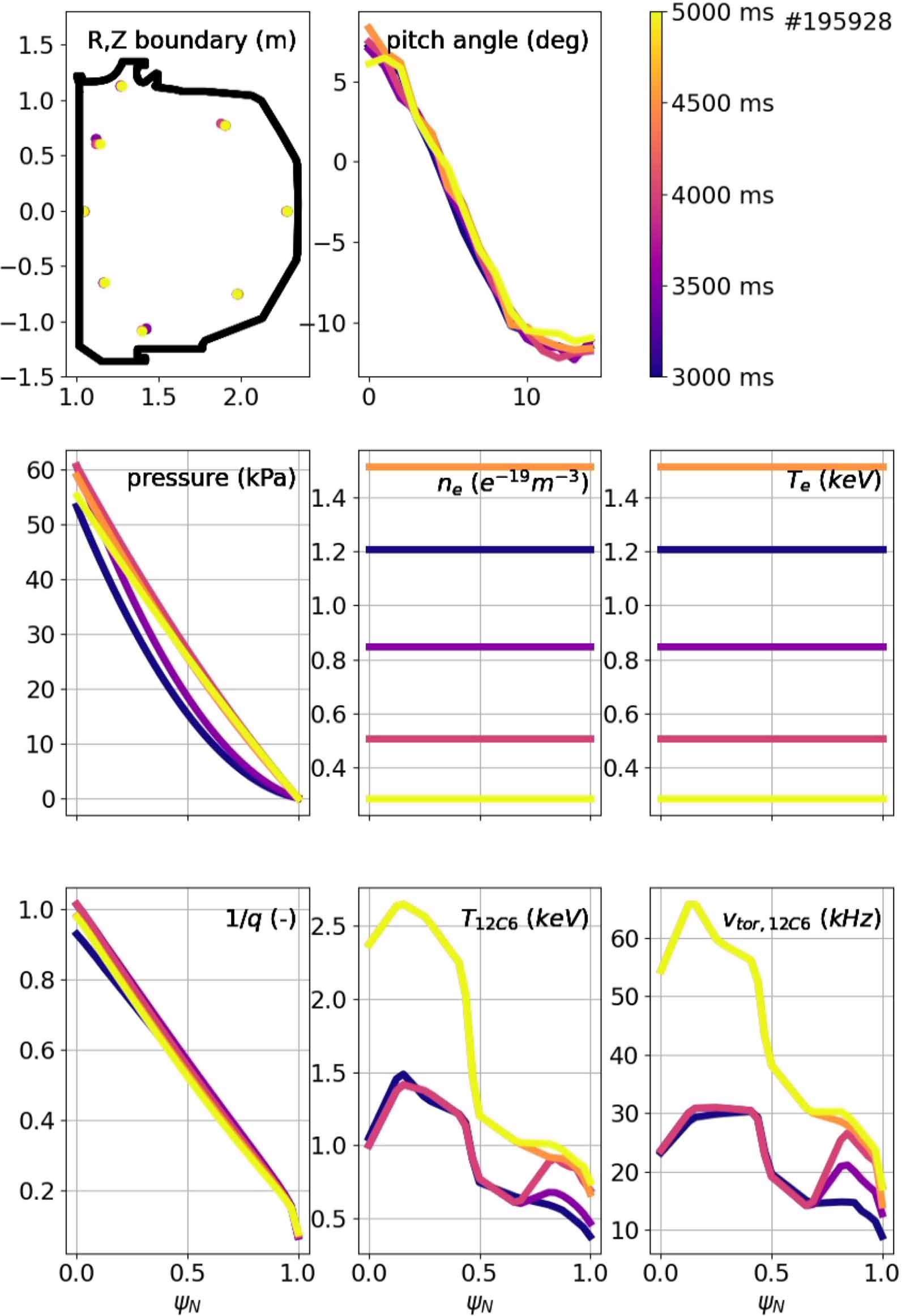
Standard image High-resolution imageFigure 9 showcases the remaining outputs generated by RTCAKENN, including the electron density and temperature profiles. Remarkably, RTCAKENN demonstrated considerable robustness in the face of missing TS data, consistently producing physically meaningful profiles. However, it is worth noting that the neural network architecture employed by RTCAKENN introduced some noticeable discontinuities in certain profiles, most notably in the toroidal velocity profile. Although an averaging method was employed to mitigate this issue by combining the outputs of ten sub-neural networks, it did not entirely eliminate the discontinuities. To overcome this limitation, the RTCAKENN architecture was subsequently modified to treat all profiles as cohesive entities, without internally separating and recombining the core and edge profiles.

Figure 9. An example of the remaining outputs generated by RTCAKENN during plasma discharge #195928 in the absence of proper Thomson scattering data. RTCAKENN still provides qualitatively accurate physical profiles, including the electron density and temperature profiles.
Download figure:
Standard image High-resolution imageIn conclusion, the application of RTCAKENN during plasma discharge #195928 demonstrated its commendable robustness in generating qualitatively accurate physical profiles, even in the absence of accurate TS data. The continuous refinement of RTCAKENN aims to enhance its robustness and accuracy, further strengthening its applicability in real-time plasma diagnostics and control.
4.2.2. RTCAKENN without CER data.
After identifying and collaborating to resolve the TS messaging issues, hardware tests were conducted for validation. As shown in figure 10, indeed we did not receive any CER data. The reason for the TS data registering as zero in the plasma core is due to the absence of horizontal data (note that the horizontal system typically provides data at even lower normalized flux coordinates than the so-called core system). As a result, the array entries designated for horizontal data remain zero and are included as such in the data used for interpolation. However, RTCAKENN is robust against this. After all, only 33 points per profile are fed to RTCAKENN, so in that sense the curve might be misleading.

Figure 10. An example of the inputs available to RTCAKENN during hardware test #914928. In this scenario, we simulate the absence of CER data.
Download figure:
Standard image High-resolution imageRTCAKENN is able to generate qualitatively accurate pressure and current density profiles in the absence of CER data, as shown in figure 11.
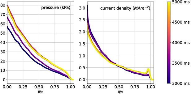
Figure 11. An example of the outputs available to RTCAKENN during hardware test #914928. In this scenario, we simulate the absence of CER data. Despite this limitation, RTCAKENN still provides qualitatively accurate physical profiles.
Download figure:
Standard image High-resolution imageSimilarly to the case where TS was absent, RTCAKENN demonstrated considerable robustness in the face of missing CER data, consistently producing physically meaningful profiles, as shown in figure 12.

Figure 12. An example of the remaining outputs generated by RTCAKENN during hardware test #914928 in the absence of proper CER. RTCAKENN still provides qualitatively accurate physical profiles, including the density and toroidal velocity profiles.
Download figure:
Standard image High-resolution imageViewing from a standpoint of robustness, it is crucial to recognize that the lack of data does not necessarily make the profiles implausible or illogical. Nonetheless, our tests specifically focused on the worst-case scenario: the total absence of TS (CER) data throughout the discharge. In practical situations, data may be intermittently received, leading to the possibility that a model could still generate reasonable profiles for various time slices even after the data input stops. However, when absolutely no TS (CER) data is received during the discharge by a model with no memory, it becomes less clear whether the model's outcomes can sustain accuracy, unless the outcome is well constrained by information embedded in other diagnostics.
While initially assessing discharge accuracy with missing TS or CER data, we could not identify distinct patterns regarding how the predictions deteriorated. For instance, when comparing electron temperature and density between RTCAKENN (using the model that treats the core and edge separately) at two time-slices, where a clear change in electron density across the profile occurred, the average discrepancy between the profiles at approximately 3500 ms (around 15%) was more significant than at 4000 ms (approximately 13%). No significant changes in magnitude were observed for other time slices during manual inspection.
With RTCAKENN becoming more regularly used and collecting additional time slices with data presence or absence, we anticipate conducting a comprehensive sensitivity analysis to map the impact of missing data on accuracy. This analysis will involve exploring the duration of data absence and assessing how effectively the model operates in the complete absence of CER or TS data.
4.2.3. RTCAKENN with different neural network architecture.
Even though plasma profile evolution often tends to be global by nature, we typically observe that in H-mode plasmas, the edge region has complex patterns with steep pressure gradients and fluctuating current density, while the core plasma has a relatively smooth shape. Due to these different spatial patterns and complexities governed by different physics mechanisms in the two regions, it is worth generating the equilibrium profiles for each region separately by different decoder networks to see if we can further enhance the accuracy of the model. This way enables each decoder network for the core and edge to focus on each dominant physical pattern.
In this section, we compare the performance of this new prediction model with a different architecture to the existing model of figure 1. Figure 13 illustrates the model structure that separates the core and edge regions based on ψN = 0.8 for decoding. Panels (a)–(c) in figure 13 remain the same as the original model, while in (d), profiles are generated for each region using separate networks and then concatenated to obtain the final profile. Figure 14 shows regression plots and error distributions using this new model. Compared to the results of the original model (figure 2), the new model demonstrates slightly lower R values and larger σ values. Furthermore, when examining a predicted profile for a specific target plasma, as shown in figure 15, there occurs a discontinuity around ψN = 0.8, the point which separates the core and edge. As the spatial gradient of the profiles plays an important role in plasma stability analysis and control, these discontinuities in the profiles can lead to significant errors in post-analysis. Considering the potential use of RTCAKENN, the original model structure in figure 1 is more suitable.

Figure 13. Neural network architecture that separates the plasma core and edge regions during the decoding process.
Download figure:
Standard image High-resolution image
Figure 14. Regression plots for the test dataset and error distributions using the trained model that separates the plasma core and edge regions. (a) Plasma pressure, (b) current density, (c) inverse of safety factor, (d) electron density, (e) electron temperature, (f) ion temperature, and (g) toroidal rotation velocity.
Download figure:
Standard image High-resolution image
Figure 15. Discontinuity of the q profile predicted by the new model, compared to 'True' value (CAKE).
Download figure:
Standard image High-resolution image4.3. Timing
Quantifying the execution time of algorithms and their constituent components in the context of a production PCS poses significant challenges due to inherent disparities between the testing and production environments. In order to gain insights into the temporal aspects of algorithm execution during each PCS cycle, including potential variations, a timing metric stored by the PCS is analyzed for each real-time function (algorithm) running on every CPU.
In this analysis, we specifically focus on examining ten neural networks that form RTCAKENN, while also taking into account associated overhead tasks such as input reception, processing, and the aggregation of outputs to derive the final results.
The results are depicted in figure 16. Two distinct bands of execution times can be visually discerned. The initial version of RTCAKENN, employed in discharge number #195928, exhibited an average execution time of approximately 13 ms, with a one-sided positive variance of 0.4 ms for the worst-case scenario.

Figure 16. Execution time of complete RTCAKENN real-time function as function of time for several plasma discharges. Note that this quantity represents the total time it takes for RTCAKENN to receive and process inputs, apply the 10 neural nets and average all outputs.
Download figure:
Standard image High-resolution image
In contrast to this, all discharges that utilized the newer version of RTCAKENN demonstrated an average execution time of approximately 7.7 ms, typically accompanied by a one-sided positive variance of about 0.1 ms. The worst-case scenario in the first cycle exhibited a deviation of 1 millisecond.
Additionally, it is noteworthy that during all of these tests, the execution times of the algorithms were significantly lower than the typical cycle time of 20 ms for the CPU (here the cycle time refers to the time a CPU can spend to complete one full cycle of its functions–not to be confused with CPU clock frequency, which is in the GHz range). This observation indicates that there were no hardware or execution issues that could potentially hinder the real-time operation of the PCS.
Furthermore, the evolution of plasma profiles typically occurs at a slower pace compared to the execution time of the algorithms. Similarly, the data provided by the diagnostics is usually available at similar or slower execution times. This synchronization between the execution time and the evolution of plasma profiles, as well as the availability of diagnostic data, ensures that the algorithmic operations are enabled to capture and represent the dynamics of the plasma.
Given the ample amount of 'unused' time within each cycle, it is evident that there is still room for incorporating additional computational complexity to enhance the performance of the algorithms. This suggests the possibility of incorporating more sophisticated algorithms to achieve enhanced control and analysis capabilities.
5. Discussion and conclusion
RTCAKENN has demonstrated its capability to generate real-time reconstructions of various plasma parameters in the DIII-D PCS, including pressure, toroidal current density, inverse q profile, electron temperature, electron density, ion carbon impurity temperature, and rotation profiles.
The quality of the profiles generated by RTCAKENN closely approximates that of the offline CAKE and typically surpasses real-time alternatives run with default settings. In practical scenarios, default settings are often utilized unless specific domain experts are involved.
As intended by its design, RTCAKENN has exhibited robustness against the absence of TS or CER data, establishing it as a valuable algorithm suitable for running during every discharge as a primary diagnostic tool for control and real-time analysis.
Currently, RTCAKENN operates efficiently on a 20 ms CPU, with the algorithm itself executing in under 8 ms.
Overall, RTCAKENN presents a promising approach to the development of a reliable tool that can operate effectively during any discharge without the need for specific setups or the availability of all diagnostics. Nevertheless, there remains room for further improvement.
It is imperative to minimize the extent of data pre-processing and shift the burden of interpretation onto the neural network. Therefore, exploring the feasibility of directly feeding RTCAKENN raw data, without resorting to linear interpolation onto a predefined ψN grid, is an active area of investigation. However, accomplishing this task is non-trivial due to the inherent challenges associated with the changing ψN values associated with TS channels or CER chords as the plasma moves. Incorporating this information into the neural network in an explicit manner poses a significant challenge.
Expanding the training dataset in terms of its size and variability, accommodating any sign of plasma current, and aligning it more closely with the observations that RTCAKENN would encounter within the PCS, are critical areas of improvement.
Further research is warranted to determine the underlying reasons for the observed variance in the regression plots pertaining to ion temperature and toroidal rotation profiles generated by RTCAKENN. Notably, the core ion temperature consistently exhibits a slightly higher value in RTCAKENN compared to CAKE.
Considering the fact that RTCAKENN executes faster than initially anticipated, there is an opportunity to introduce additional computational complexity to further enhance the accuracy and robustness of the algorithm, albeit at the expense of timing. However, given that certain inputs do not refresh faster than every 20 ms and plasma profiles generally evolve on similar or slower timescales, sacrificing a certain degree of speed in favor of improved robustness and accuracy represents the optimal course of action for both control and real-time analysis applications.
Acknowledgments
This work was supported by the National Research Foundation of Korea(NRF) funded by the Korea government. (Ministry of Science and ICT) (RS-2023-00255492). This material is based upon work supported by the US Department of Energy, Office of Science, Office of Fusion Energy Sciences, using the DIII-D National Fusion Facility, a DOE Office of Science user facility, under Award DE-FC02-04ER54698. In addition this material was supported by the US Department of Energy, under Awards DE-SC0015480 and DE-AC02-09CH11466.
Disclaimer
This report was prepared as an account of work sponsored by an agency of the United States Government. Neither the United States Government nor any agency thereof, nor any of their employees, makes any warranty, express or implied, or assumes any legal liability or responsibility for the accuracy, completeness, or usefulness of any information, apparatus, product, or process disclosed, or represents that its use would not infringe privately owned rights. Reference herein to any specific commercial product, process, or service by trade name, trademark, manufacturer, or otherwise does not necessarily constitute or imply its endorsement, recommendation, or favoring by the United States Government or any agency thereof. The views and opinions of authors expressed herein do not necessarily state or reflect those of the United States Government or any agency thereof.
Appendix: Encoding networks
Three encoder networks shown in figure 1(b) receive different kinds of input signals to extract features in reduced dimensions. In all the encoder networks, batch normalization is applied before each hidden layer to redistribute the features, and the ReLU activation is applied after each layer to provide nonlinearity.
The pitch angle encoder network consists of fully connected layers. This MLP has three layers, each with 16, 8, and 4 neurons, respectively, which encodes 15 pitch angle signals into four features. The boundary encoder network also consists of three fully connected layers, each with 32, 16, and 8 neurons, respectively. This encodes the boundary coordinate information of 16 parameters into eight features. Lastly, the kinetic encoder network consists of two 1D convolutional layers. Each convolutional layer has 16 and 32 neurons, respectively, with a kernel of size 3. After each convolutional operation, max pooling of size 2 is applied to reduce the dimension. After the profile encoding, the reduced features are flattened and passed through a fully connected layer of 64 neurons.
Decoding networks:
The extracted input features are concatenated and passed through the latent feature extraction network shown in figure 1(c). The latent feature extractor has two fully connected layers, each with 128 neurons.
Lastly, from the 128 latent features, the decoding network (figure 1(d)) reconstructs the final 1D profiles. The network has three blocks, each operates one 1D upsampling and two 1D convolutions sequentially. The convolutional layers has 64, 16, 32, and 7 neurons each, finally generating seven 1D profiles.