


Abstract
Spatially resolved rotational temperature of ground state hydrogen molecules desorbed from plasma-facing surface was measured in QUEST, LTX-β, and DIII-D tokamaks, and the increases of the rotational temperature with the surface temperature and due to collisional-radiative processes in the plasmas were evaluated. The increase due to collisional-radiative processes was calculated by solving rate equations considering electron and proton collisional excitation and deexcitation and spontaneous emission. The calculation results suggest a high sensitivity for the rotational temperature to electron and proton densities, but a negligible sensitivity to the electron, proton, and surface temperatures. In the three tokamaks with different plasma parameters and plasma-facing surface materials, the spatial profile of the rotational temperature was estimated using Fulcher-α emission lines (600–608 nm). In QUEST, the spatial profile of the rotational temperature was estimated from spatially resolved spectra. In the other tokamaks, the rotational temperature was evaluated assuming a single point emission with a location determined from the Fulcher-α emission profile as measured with a filtered camera. In metal-walled devices QUEST and LTX-β, the rotational temperature increased with the surface temperature, and the calculated collisional-radiative increase is consistent with measured increase assuming that the rotational temperature at the surface is approximately 500–600 K higher than the surface temperature. In DIII-D with carbon walls, a larger collisional-radiative increase than the other tokamaks was observed because of the higher density leading to a large difference from the calculated increase compared to the other smaller tokamaks. Measurement of the Fulcher-α emission profile with higher spatial resolution in DIII-D may reduce the difference and reveal the effect of the surface temperature on the rotational temperature. These results show the increases in the rotational temperature with the surface temperature and due to the collisional-radiative processes.
Export citation and abstract BibTeX RIS

Original content from this work may be used under the terms of the Creative Commons Attribution 4.0 license. Any further distribution of this work must maintain attribution to the author(s) and the title of the work, journal citation and DOI.
1. Introduction
In a tokamak fusion device, hydrogen molecules are produced by the recombination of impinging H+ ions and neutrals within the first layers of the plasma-facing surface, then re-released by thermally-driven processes into the plasma in a process known as recycling. The recycled molecules affect detachment of the divertor plasma, or a reduction of the heat and particle flux to the surface, via the process of molecular assisted recombination (MAR) in the near-surface plasma. Dissociative attachment is one of the MAR processes with the rate which is dependent on the rovibrational state of the molecules [1]. Thus, rovibrational population distribution of the recycled molecules is an important parameter. This paper focuses on the rotational temperature, which can be evaluated from the measurement with existing spectrometers for a plasma shot, and describes the investigation of the hydrogen molecular rotational temperature near the plasma-facing surface.
In a tokamak edge plasma with sufficient temperature to maintain ionized hydrogen, those ions move along the magnetic field line, are charge neutralized on the surface, recombine with other neutral hydrogen atoms within the surface, and are desorbed as atoms and molecules. These processes are schematically shown in figure 1. The rovibrational temperatures of the desorbed molecules are affected by both the surface temperature of the walls  and the excitation resulting from recombination processes which occur within the plasma-facing surface. One of those processes, the Eley–Rideal recombination, is exothermic by about 2.3 eV. Previous experimental work revealed that this process rovibrationally excites the molecules which then desorb [2]. The desorbed molecules enter the plasma and collide with electrons and protons. The collisions affect the rovibrational temperatures of the desorbed molecules via collisional-radiative processes.
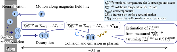
Figure 1. Processes affecting the rotational temperatures of hydrogen molecules near the plasma-facing surface.
Download figure:
Standard image High-resolution imageAn increase in the rotational temperature with  and electron density
  near the plasma-facing surface were observed for deuterium discharges in TEXTOR [3, 4] and DIII-D [5]. In TEXTOR, the rotational temperature of desorbed molecules near the graphite test limiter was measured, and its increase with the limiter temperature and
  at the last closed flux surface (LCFS) [3, 4] was evaluated. In DIII-D, the rotational temperature for the d3Π state
  near the graphite target in the lower divertor and its increase with the local electron density
  [5] were measured. Assuming that
  is equal to the ratio of the molecular constants
  2 [6], i.e.
 , the estimated
  from [5] approached a temperature close to but
  300–400 K higher than
  (
( 400–500 K) when
  tends to zero, where
  denotes the electronic ground state, and
  and
and  represent the vibrational quantum numbers (see markers and a gray line in figure 2). The increase in
  with
with  and the convergence to a higher temperature than
  , which are shown in these early studies, infer that
  of the desorbed molecules can be affected by surface effects: surface temperature
  and excitation due to recombination of neutral hydrogen atoms to molecules (
 ), respectively. The increase with
  implies an effect due to collisional-radiative processes in the plasma (
 ).
).
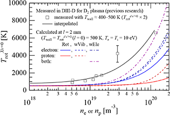
Figure 2. Measured and calculated  . The markers show
  measured in DIII-D with
  400–500 K [5] multiplied by two assuming a relation
  . The gray line shows a fit to the measured results [5]. The other lines show the rotational temperature resulting from each process as calculated by our model described in section 2 with the conditions
  500 K,
  10 eV. Colors of the lines show models considering electron (blue), proton (red), and both (purple) collision processes. Solid, dashed, and chain lines show the calculation results using the model considering only pure rotational, rovibrational, and rovibronic excitation and deexcitation, respectively (see table 2).
Download figure:
Standard image High-resolution imageIn order to evaluate these effects on  , the results of this paper demonstrate a calculation of
  and spatially presents resolved measurements of
  . The rotational temperature is usually different for different vibrational states, and that for the vibrational ground state (
 0)
0)  was examined. A comparative study was made using three tokamaks of different plasma parameters and surface materials: QUEST, LTX-β, and DIII-D. Section 2 describes a model developed for the evaluation of
  , and section 3 shows experimental results and their comparison with results from computational models.
2. Calculation
2.1. Modeling of collisional-radiative processes
Collisional-radiative processes of hydrogen molecules were modeled assuming that molecules were desorbed from the plasma-facing surface and moved perpendicular to the surface with a velocity  . A one-dimensional coordinate system
  perpendicular to the plasma-facing surface and directed toward the plasma is introduced to describe the motion of the molecules. The origin of the
  -axis is on the surface. The velocity of molecules
  was assumed to be constant since the mean free paths for the momentum transfer due to collisions with electrons, protons, hydrogen atoms, and hydrogen molecules are longer than the spatial scales in the plasma considered later in this paper [7, 8].
In the plasma, the rotational population distribution for the ground state (X1Σg
+) of hydrogen molecules can be modified by the following collisional-radiative processes: (i) excitation, (ii) deexcitation, (iii) spontaneous emission, (iv) dissociation, (v) ionization, (vi) recombination of electron and hydrogen molecular ions, (vii) charge exchange, and (viii) electron attachment. In this study, processes (i) and (ii) by electron and proton collisions and (iii) were considered, and the other processes (iv)–(viii) were neglected for reasons discussed below. Processes (i) and (ii) by collisions with hydrogen atoms and molecules were neglected because of their small population fluxes at the plasma parameters of this study. For instance, the population fluxes of the pure rotational excitation by collisions with electrons, protons, hydrogen atoms, and hydrogen molecules, are estimated to be ∼1019, 1018, 1016, and 1014 m–3 s–1, respectively, for representative parameters in QUEST;  1017 m–3,
  1016 m–3,
  1016 m–3,
  5 eV,
5 eV,  2.5 eV,
  1.5 eV, and
  300 K [9]. In LTX-β and DIII-D, the relative population fluxes have comparable orders to that of the example. Process (iv) consists of the dissociation by rovibrational excitation in the ground state and that by excitation to repulsive state b3Σu
+. The former has larger effect on the population for higher vibrational states due to a larger cross section. Therefore, the effect of the former can be evaluated by reducing the number of rovibrational states considered in a model. This only changes
300 K [9]. In LTX-β and DIII-D, the relative population fluxes have comparable orders to that of the example. Process (iv) consists of the dissociation by rovibrational excitation in the ground state and that by excitation to repulsive state b3Σu
+. The former has larger effect on the population for higher vibrational states due to a larger cross section. Therefore, the effect of the former can be evaluated by reducing the number of rovibrational states considered in a model. This only changes  by a comparable value to the uncertainty of the evaluated
  for the parameters in the three tokamaks. Processes (v) by electron collisions and (vii) have cross sections comparable to those for the electron and proton collisional rovibrational excitations, respectively, and can affect the rotational population distribution [9, 10]. However, these processes were neglected since the rotationally resolved cross section data are not available. When they have no rotational dependence, the effects of these processes are expected to be small because of no direct effect on the rotational temperature for each vibrational state. The effects of the processes (vi) and (viii) are unknown because of the absence of valid data.
The spatial profile of the rovibrational population for the ground state  was derived by solving the rate equations. Here,
  is the rotational quantum number, and
  is population of the state denoted by
  , where the bracket denotes the set of the electronic state and rovibrational quantum numbers. Assuming steady state, the spatial derivative of
  can be described by the temporal variation in
  for molecules during their travel from the surface:
The right-hand and left-hand sides are in Lagrangian and Eulerian descriptions. Note that the reflection of the molecules on the wall was ignored in the model. The spatial profile of  was derived by solving differential equations (rate equations) as described by
where  denotes a virtual electronic excited state,
  is the Einstein A coefficient for the spontaneous transition from
  to
to  , and
, and  and
and  are the rate coefficients for collisional excitation and deexcitation, respectively, from
  to
to  . The subscripts 'e' and 'p' indicate the collision with electrons and protons, respectively, and the rate coefficients depend on their temperatures. The first term in the right-hand side of equation (2) includes the spontaneous transition and excitation by the electron collisions between the X state and
  state. Bundled B1Σu
+, B'1Σu
+, C1Πu, and D1Πu states were considered as
state. Bundled B1Σu
+, B'1Σu
+, C1Πu, and D1Πu states were considered as  state because of their largest excitation fluxes from the X state [11]. The second and third terms are electron collisional excitation and deexcitation in the X state. The second term is the excitation from and deexcitation to the lower states. The third term is the excitation to and deexcitation from the upper states. The fourth and fifth terms are due to the proton collisions. Note that the pure rotational and rovibrational excitation and deexcitation in the
  state were ignored because of the long time scale of the collisional excitation and deexcitation compared to the lifetime of the e' state, determined by the spontaneous emission. The above equations were solved for rovibrational states with 0
  14 and 0
  25 for the
  state and the rovibrational states with 0
  17 and 0
  25 for the
  state. Namely 858 simultaneous differential equations were solved. The spatial profiles of
  ,
,  ,
,  , and
, and  are given, and their arguments are converted time by using the relation
  .
.
The adopted dataset for the cross sections and the Einstein A coefficients is summarized in table 1. Some of the cross sections are shown in figure 3. No processes changing the nuclear spin of hydrogen molecules were considered. The rate coefficients of electron collisional excitation are ∼10 times higher than those of proton collisional excitation when the densities of protons and electrons are equal and  5–40 eV. The processes considered in the model and their cross sections are explained in detail in the supplementary data.

Figure 3. Cross sections for rovibrational excitation from H2 X state by electron (e) and proton (p) collisions [7, 12, 13]. The extrapolated data are shown by dashed lines when data were not available up to 500 eV.
Download figure:
Standard image High-resolution imageTable 1. Summary of cross sections and Einstein A coefficients.
| Pure rotational excitation by electron collisions | |
|---|---|
( 0, 0,  0–1) → ( 0–1) → ( 0, 0,  ) ) | [12] |
( 0, 0,  2) → ( 2) → ( 0, 0,  2) 2) | Same as ( 0, 0,  1) → ( 1) → ( 0, 0,  3) 3) |
( 1, 1,  ) → ( ) → ( , ,  2) 2) | Same as ( 0, 0,  ) → ( ) → ( 0, 0,  2) 2) |
| Rovibrational excitation by electron collisions | |
( 0, 0,  ) → ( ) → ( 1–7, 1–7,  ) ( ) ( 1–7, 1–7,  ) → ( ) → ( 1 1  8, 8,  ) ( ) ( 9–13, 9–13,  ) → ( ) → ( 1 1  14, 14,  ) ) | Calculated using method in [13] |
( 1–8, 1–8,  ) → ( ) → ( 9–13, 9–13,  ) ) | Derived from deexcitation cross sections calculated using method in [13]. |
( , ,  ) → ( ) → ( , ,  ),
where ),
where  is the maximum rotational quantum number of the available cross sections for ( is the maximum rotational quantum number of the available cross sections for ( , ,  ) → ( ) → ( , ,  ) )
| Same as ( , ,  ) → ( ) → ( , ,  ) ) |
( , ,  ) → ( ) → ( , ,  2) 2) | Same as ( , ,  ) → ( ) → ( , ,  ) ) |
| Rovibronic excitation by electron collisions | |
( , ,  0) → ( 0) → ( )( )( , ,  0) → ( 0) → ( )
( )
( , ,  0) → ( 0) → ( )
( )
( , ,  0) → ( 0) → ( ) )
| [14], vibrationally resolved by multiplying the Franck–Condon factors in [15] and rotationally resolved assuming no rotational dependence following procedure adopted in [9] |
( , ,  0) → ( 0) → ( ), ( ), ( ), ( ), ( ), or ( ), or ( ) ) | Same as ( , ,  0) → ( 0) → ( ), ( ), ( ), ( ), ( ), or ( ), or ( ) and rovibrationally resolved ) and rovibrationally resolved |
| Pure rotational excitation by proton collisions | |
( 0, 0,  0–1) → ( 0–1) → ( 0, 0,  2) 2) | [7] |
( 0, 0,  2) → ( 2) → ( 0, 0,  2) 2) | Same as ( 0, 0,  1) → ( 1) → ( 0, 0,  3) 3) |
( 1, 1,  ) → ( ) → ( , ,  2) 2) | Same as ( 0, 0,  ) → ( ) → ( 0, 0,  2) 2) |
| Rovibrational excitation by proton collisions | |
( 0, 0,  0) → ( 0) → ( 1–3, 1–3,  0) 0) | [7] |
( 1–5, 1–5,  0) → ( 0) → ( 1, 1,  0) 0) | Scaled from cross section for ( 0, 0,  0) → ( 0) → ( 1, 1,  0) by multiplying ratio of electron collisional excitation cross section for ( 0) by multiplying ratio of electron collisional excitation cross section for ( , ,  0) → ( 0) → ( 1, 1,  0) to that for ( 0) to that for ( 0, 0,  0) → ( 0) → ( 1, 1,  0) at 4 eV in [16] following procedure adopted in [9] 0) at 4 eV in [16] following procedure adopted in [9] |
( , ,  ) → ( ) → ( , ,  ) ) | Same as ( , ,  ) → ( ) → ( , ,  ) ) |
| Einstein A coefficient for rovibronic deexcitation | |
( , ,  , ,  ) → ( ) → ( , ,  , ,  1) ( 1) ( , ,  , ,  ) → ( ) → ( , ,  , ,  1) ( 1) ( , ,  , ,  ) → ( ) → ( , ,  , ,  1) ( 1) ( , ,  , ,  ) → ( ) → ( , ,  , ,  1) 1) | [17] |
( , ,  , ,  ) → ( ) → ( , ,  , ,  1) not given by [17] 1) not given by [17] | Scaled from cross section for ( , ,  , ,  ) → ( ) → ( , ,  , ,  ) by multiplying ratio of Hönl–London factors in [18, 19] ) by multiplying ratio of Hönl–London factors in [18, 19] |
2.2. Evaluation of collisional-radiative increase in rotational temperature
The spatial profile of the rotational temperature  was evaluated by solving the rate equations (equation (2)). The initial conditions, parameters at
  0, are given as follows:
  follows a Boltzmann distribution at
  ,
,  0, and
  , where
  is the mass of a hydrogen molecule. The Boltzmann distribution is described by the following equation:
where  is the population of the X state, which is equivalent to the hydrogen molecular density,
  is the population of the vibrational state denoted by the quantum number
  ,
,  and
and  are the inverse of the vibrational and rotational partition functions, respectively,
  is the multiplicity of the rotational state,
  is the spin multiplicity of the nuclei, and
  and
and  are the vibrational and rotational energies of the X state, respectively. The vibrational energy
  is taken from [15]. The rotational energy
  was calculated using the polynomial approximation [20] and the molecular constants were taken from [21]. With these initial conditions and given
  and spatial profiles of
  ,
,  ,
,  , and
, and  , the rate equations (equation (2)) are solved using the forward Euler and Runge–Kutta methods for the first term and the other terms, respectively. The time step of
  10–9 s was adopted because the change in
  due to
  was small. Every 100 time steps of the calculation,
  was evaluated from the calculated rotational population distribution
  by fitting the populations in the states with
  0 and
0 and  5 to equation (3) according to the procedure used for the analysis of the experimental data. The model developed for the evaluation of
  was benchmarked using conditions of thermal equilibrium and the results of a rovibrationally unresolved collisional-radiative calculation code [11]. The method and results of the benchmark are described in the supplementary data.
The dependences of  on
on  ,
,  ,
,  ,
,  ,
,  and
and  were investigated assuming uniform profiles of the plasma parameters. The calculated
  is plotted as a function of
  in figure 4 for a
  distance of up to 5 cm from the surface, where the left and right columns show the effects of the electron collisional and radiative processes (
 0) and proton collisional processes (
 0), respectively. Figures 4(a)–(c) show the dependences on (a)
  , (b)
, (b)  , and (c)
  , and figures 4(d)–(f) show the dependences on (d)
  , (e)
, (e)  , and (f)
  . The values of the fixed parameters were set to
  1018 m–3,
  1018 m–3,
  10 eV,
  10 eV, and
  500 K. The calculated
  increased with
  , which is natural that the longer
  provides greater opportunity for collisional excitation. The calculated
  is nearly proportional to
  for the parameters considered here. Among the other parameters,
  and
and  are most sensitive parameters for
  and
and  is nearly proportional to them. The dependence on
  is small, as a result of the small variation in the cross sections for
  5 eV. For proton collisional processes, the cross sections for pure rotational excitation are more than 10 times larger than those for vibrational excitation when
  10 eV, and this results in the different dependence on
  when
when  10 eV or
  10 eV. The dependence on
  is negligible for both electron and proton collisional processes.
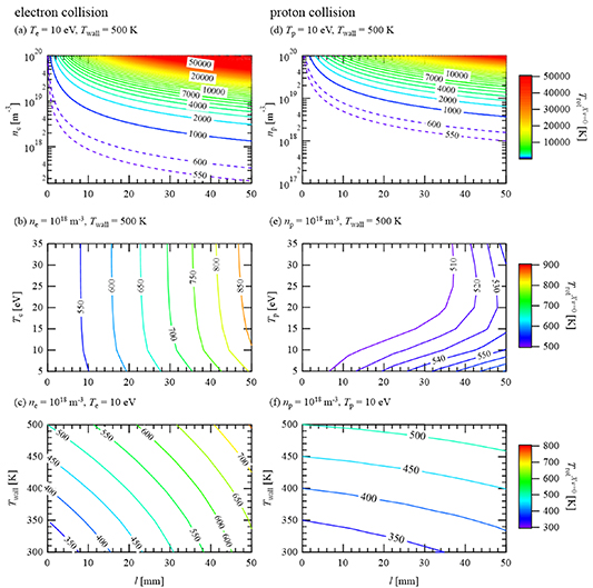
Figure 4. Calculated  plotted as a function of
  . Left column shows
  calculated for the model considering electron collisional and radiative processes (
 0) with different (a)
  , (b)
, (b)  , and (c)
  conditions. Right column shows that calculated for the model considering proton collisional processes (
 0) with different (d)
  , (e)
, (e)  , and (f)
  conditions. The same color scale is used for the figures in the same rows. A logarithmic color scale is used in the first row because
  take much higher temperature than those in the other rows.
Download figure:
Standard image High-resolution imageThe effects of the collisional-radiative processes on the increase in  were compared for
  and/or
  1018–1020 m–3. Figure 2 shows the calculated
  at
at  2 mm plotted versus
  and/or
  . The colors of the lines represent the results for the model considering electron (blue), proton (red), and both (purple) collisions, where the combination is close to a simple sum of electron and proton contribution. Solid, dashed, and chain lines show the results using the model considering the rotational (Rot), rovibrational (wVib), and rovibronic (wEle) excitation and deexcitation processes, respectively (see table 2). Among these reactions, the rovibronic and rovibrational transitions become effective when the product of the density (
 or
or  ) and
) and  exceeds 1017 m–2. The product is proportional to the number of collisions. When the number of the collisions is small, the population fluxes of vibrational and electronic deexcitations is small compared to those of excitations. This results in the small effect of the vibrational and electronic excitations on
  .
.
Table 2. Processes considered in the model. Check marks show the processes considered in the model labeled 'Rot', 'wVib', and 'wEle', respectively.
| Processes | Rot | wVib | wEle | |
|---|---|---|---|---|
| By electron collisions | Pure rotational excitation/deexcitation | ✔ | ✔ | ✔ |
| Rovibrational excitation/deexcitation | ✔ | ✔ | ||
| Rovibronic excitation/deexcitation | ✔ | |||
| By proton collisions | Pure rotational excitation/deexcitation | ✔ | ✔ | ✔ |
| Rovibrational excitation/deexcitation | ✔ | ✔ |
3. Experiment
3.1. Experimental setup
The ground state rotational temperature of hydrogen molecules  was measured in three tokamaks: QUEST, LTX-β, and DIII-D. The schematic illustrations of their poloidal cross sections are shown in figure 5. QUEST (Q-shu University Experiment with Steady-State Spherical Tokamak) is a spherical tokamak shown in figure 5(a). The major and minor radii are 0.64 m and 0.46 m, respectively. The vacuum vessel and plasma-facing components are made of stainless steel. The plasma-facing components called 'hot walls' are coated with atmospheric plasma-sprayed tungsten (APS-W) and have heaters to control the surface temperature [22]. LTX-β (Lithium Tokamak Experiment Beta) is a spherical tokamak shown in figure 5(b). The major and minor radii are 0.40 and 0.26 m, respectively. The plasma-facing components called 'shells' are made of a 1-inch-thick copper plate clad with stainless steel conformal to the LCFS. The plasma-facing surface of the shells was coated with lithium using evaporators at two toroidal locations, and the lithium condition was maintained either in the solid or liquid phase by adjusting the shell temperature using heaters. DIII-D (Doublet III-D) is a tokamak shown in figure 5(c). The major and minor radii are 1.7 and 0.6 m, respectively. The vacuum vessel is made of Inconel, and the plasma-facing components are mostly armored with ATJ graphite and partly with carbon fiber composite tiles [23]. QUEST and LTX-β use a limiter configuration, and DIII-D uses a divertor configuration. Plasmas were produced and sustained by 28 GHz electron cyclotron resonance heating in QUEST [24], ohmic heating in LTX-β, and ohmic heating and neutral beam injection in DIII-D. The LCFSs of the plasmas are shown by thick gray lines in figure 5. For the data analyzed here, all devices utilized attached L-mode hydrogen plasmas.
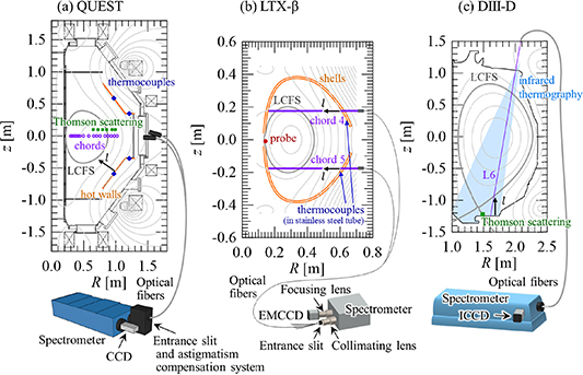
Figure 5. Magnetic equilibria and the spectroscopic systems used for (a) QUEST, (b) LTX-β, and (c) DIII-D. Viewing chords are shown by purple markers in (a) and purple lines in (b) and (c). Measurement positions of Thomson scattering and a probe are shown by green squares and a red circle, respectively. Note that the green squares in (a) QUEST are shifted upward to avoid overlap with the purple markers.
Download figure:
Standard image High-resolution imageThe surface temperatures of the plasma-facing components were measured with thermocouples in QUEST and LTX-β and using IR thermography in DIII-D. In QUEST, four thermocouples are installed at the back side of the hot walls at the positions indicated by the blue diamonds in figure 5(a). In LTX-β, two thermocouples are mounted in stainless steel tubes which are welded to the shell, on the outboard side, and exposed to plasma. The temperatures measured with the thermocouples were regarded as representative of the surface temperatures given the small deposited energy away from the limiter. In DIII-D, an infrared camera looking at the lower divertor target plate was used to measure the spatial profile of the surface temperature of the plasma-facing components. The field of view is shown in blue in figure 5(c). The measured temperatures were regarded as the surface temperatures.
The electron density and temperature were measured with Langmuir probes or by Thomson scattering. In QUEST, the radial profiles of  and
and  were measured in the outboard midplane by Thomson scattering [25], and the measurement positions are shown by the green squares in figure 5(a). In LTX-β, local
  and
and  were measured with a Langmuir probe on the inboard side of the shells, which is shown by the red circle in figure 5(b). Note that the probe, while at the same normalized flux coordinate, was in a magnetically disconnected region and the measured values could differ from those at the positions where the rotational temperatures were measured. In DIII-D, local
  and
and  were measured by Thomson scattering near the lower divertor target plate as shown by a green square in figure 5(c).
3.2. Spectroscopic systems
The Q-branch rotational line spectra belonging to the Fulcher-α band (d3Πu,  0 → a3Σg
+,
0 → a3Σg
+,  0, 600–608 nm) were measured to derive the d and X state rotational temperatures of hydrogen molecules. The spectroscopic systems with high spectral resolutions utilized in this work are schematically illustrated in figure 5. Each spectroscopic system consists of optical fibers, a spectrometer, and a charge coupled device (CCD) camera. The optical fibers were used with collimators and collected emission from the plasma. The collected emission enters a spectrometer through an entrance slit, and the dispersed spectra were recorded on a CCD camera. In QUEST, 16 tangentially-viewing optical fibers with 0.25 mm core diameters were used with two achromatic lenses. The fibers were connected to a Czerny–Turner spectrometer (Acton Research, AM-510; 1 m focal length, F/8.7, and 1800 grooves mm−1 grating), and the spectra were recorded on a CCD camera (Andor Technology, DU440-BU2; 2048
  512 pixels and 13.5 μm square pixels) [26]. In LTX-β, two radially-viewing optical fibers with 0.6 mm core diameter were used with reflective collimators. The optical fibers were connected to a lens-based spectrometer [27] which consists of two camera lenses for collimating and focusing (Canon 200 mm f/1.8 EF) and a grating with 2160 grooves mm−1. The spectra were recorded on an electron multiplying CCD camera (Princeton Instruments, ProEM 512; 512
  512 pixels and 16 μm square pixels) [27]. In DIII-D, one of the six vertically viewing optical fibers, part of the multi-chord divertor spectrometer system [28], with 0.6 mm core diameter was used, looking at the lower divertor. The fibers are connected to a Czerny–Turner spectrometer (McPherson Corporation, Model 209; 1.33 m focal length, F/11.6, and 1200 grooves mm−1 grating) [28]. The dispersed spectra were recorded on an intensified CCD camera (Princeton Instruments, PI-MAX4 1024i; 1024
  1024 pixels and 12.8 μm square pixels).
The viewing chords were aligned to measure the emission near the plasma-facing walls. They are shown in purple with the poloidal cross-sectional views of the devices in figure 5. In QUEST, the viewing chords were aligned on the midplane, and the tangency radii of the viewing chords  are shown by the purple markers [26]. The diameters of the viewing chords were approximately 30 mm at the tangency plane. In LTX-β, two viewing chords were aligned almost radially as shown by the purple lines, and the diameters of the viewing chords were approximately 30 mm on the shells. In DIII-D, the viewing chord named L6 was used as shown by the purple line. The diameter of the viewing chord was 22 mm on the divertor target plate.
The wavelength and radiance of the observed spectra were absolutely calibrated, and the instrumental functions of the systems were evaluated. The instrumental functions of the systems were regarded as a Gaussian function. Their FWHMs were approximately 0.07, 0.07, and 0.04 nm for the systems in QUEST, LTX-β, and DIII-D, respectively.
3.3. Evaluation of rotational temperatures
The rotational temperatures of the d and X state were evaluated from the measured Q-branch rotational line spectra. The spectra are shown by the black markers, and their central wavelengths by the purple vertical lines in figure 6. The latter were identified with a data table [29].

Figure 6. Measured and fitted spectra in (a) QUEST, (b) LTX-β, and (c) DIII-D. Black markers and magenta lines show the measured spectra and fitted spectra with Gaussian functions, respectively. Purple vertical lines show the central wavelength of the Q-branch rotational lines [29]. Gray boxes below the spectra show the fitting range.
Download figure:
Standard image High-resolution imageFor the spectra measured in QUEST, the radial profiles of Q1–Q5 line emissivity were evaluated assuming their toroidal symmetry. Firstly, the measured Q1–Q5 line spectra were fitted to Gaussian functions as shown by the magenta line in figure 6(a), and the chord-integrated radiance  of each line was derived. The measured
  is shown by markers in figure 7(a). Then, their continuous tangential profiles were evaluated by fitting to sigmoid functions, which well reproduce the
  -dependences of the measured
  in the region of our interest
  0.7 m. The fitted
  profiles are shown by lines in figure 7(a). Lastly, the Abel inversion was applied to the fitted
  assuming the toroidal symmetry of the plasma, and the radial profiles of the emissivity were obtained as shown in figure 7(b). The error of the emissivity was estimated by the following four steps [26]: (I) generate 500 datasets by adding Gaussian noise with the estimated standard deviation of
  to the measured
  , (II) fit each dataset to a sigmoid function, (III) apply the Abel inversion to the fitted dataset, and (IV) calculate the mean and standard deviation of the derived emissivity at each radial position. The mean and standard deviation were plotted as the value and standard deviation of emissivity in figure 7(b). Note that the fitted
  profiles and their error are also derived from the mean and standard deviation of 500 fitted dataset produced in step (II).
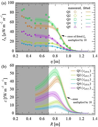
Figure 7. (a) Chord-integrated radiance  and (b) emissivity
  of the Q1–Q5 lines evaluated from the spectra measured in QUEST. The data in the shaded ranges was not used for the analysis.
Download figure:
Standard image High-resolution imageFor the spectra measured in LTX-β and DIII-D, where view have no toroidal component, emissivity of the Q1–Q5 lines were evaluated assuming single point emissions because the Fulcher-α emission is localized near the plasma-facing walls due to larger spatial gradients of the  and
and  . The Q1–Q5 line spectra measured in LTX-β were fitted to Gaussian functions as shown by the magenta line in figure 6(b). For the spectra measured in DIII-D, the Zeeman splitting was observed in the Q1 line spectrum (figure 8(a)) because of a larger magnetic field (∼2 T) than the other two devices [30], and a symmetric triple Gaussian function was used to approximate the spectrum. Additionally, the Q3 line spectrum overlapped with the other lines, one of which was a hydrogen molecular line at 603.1465 nm. We assumed three overlapping lines and separated the Q3 line spectrum as shown in figure 8(b). The other line spectra were fitted to Gaussian functions as shown by the magenta line in figure 6(c).
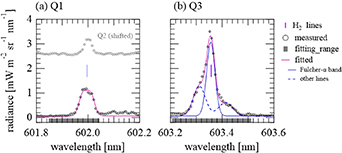
Figure 8. Enlarged spectra near the central wavelength of (a) Q1 and (b) Q3 lines measured in DIII-D. Q2 line is also plotted in (a) for comparison. For the Q1 line, broadening by Zeeman splitting was observed. For the Q3 line, three overlapping lines were separated by fitting to a triple Gaussian function. The separated Q3 line spectrum and the contaminant line spectra are shown by the blue solid and dashed lines, respectively.
Download figure:
Standard image High-resolution imageThe localization of the Fulcher-α emission near the plasma-facing surface in LTX-β and DIII-D was confirmed by wavelength filtered camera images. In LTX-β, the wavelength-integrated irradiance at  0.176 m corresponding to the height of chord 5 was evaluated from the camera image (figure 9(a)) as shown in figure 9(b). The irradiance is localized and peaks near the wall. Since the peak position of the emissivity is expected to be ∼30 mm (
 10 pixels) away from the shell surface, the Fulcher-α emission was approximated as a point source at the distance of 0.03 m from the shell surface. In DIII-D, the emissivity profile in a poloidal plane was reconstructed from the Tangential TV diagnostics [31] shown in figure 10(a) in a deuterium discharge with the same operational condition as the discharge used in this work. The emissivity profile along the adopted viewing chord (L6) as a function of
  was calculated as shown in figure 10(b). The reconstructed emissivity is localized near the outer target plate, and the Fulcher-α emission was approximated as a point source at the distance of 0.01 m from the surface of the target plate, where the emissivity is peaked. This was also confirmed by the emissivity profile derived from a simulation by EDGE2D-EIRENE [32] (see figure 10(c)).

Figure 9. (a) Irradiance profile of Fulcher-α band measured in LTX-β with a wavelength filtered camera (602.36 nm central wavelength and 2.43 nm FWHM) for  297 K (solid lithium surface). The camera was directed radially. The brightest emission on the right side of the center stack is due to gas injection. (b) Irradiance profile along chord 5, the horizontal solid line shown in (a), considering its width shown by the horizontal dashed lines. The viewing chords in the range of 0–3 horizontal pixels could be disturbed by the edge of the window and 55–60 horizontal pixels are terminated by the center stack.
Download figure:
Standard image High-resolution image
Figure 10. (a) Emissivity profile of Fulcher-α band obtained in a low-density deuterium L-mode discharge in DIII-D (#174235) from inversion of a wavelength filtered tangentially-viewing camera image in the lower divertor (601.8 nm central wavelength and 2.8 nm FWHM) [31]. (b) Emissivity profile along a viewing chord as a function of  when
when  0.04 m, where
  is a distance from the outer strike point to the intersection of a viewing chord and the lower divertor target plate. (c) Emissivity profile along a viewing chord with
  0.02 m derived from a simulation by EDGE2D-EIRENE [32].
Download figure:
Standard image High-resolution imageThe rotational temperature for the  state was derived from the relative intensities of the Q1–Q5 lines. When the rotational population distribution follows a Boltzmann distribution, the population divided by the statistical weight can be expressed by the following equation, so-called Boltzmann plot:
where  ,
,  , and
, and  are the rotational population, energy, and temperature, respectively, of the
  state. The population in the states with
  0 and
0 and  5 was used to evaluate
  since it was well approximated to a Boltzmann distribution in a DIII-D plasma [5].
The population  was evaluated from the measured emissivity of the Q1–Q5 lines
  divided by a factor
  , which is proportional to the Einstein A coefficient. Here,
  is the Hönl–London factor and is given by
  . Thus, equation (4) can be written
and  is determined from the slope of this logarithmic plot versus
  as shown in figure 11. For the results in QUEST, the error of
  shown in the figures includes no systematic errors of Abel inversion coming from the toroidal asymmetry of the emissivity profile and low accuracy of measured
  for larger
  . They were estimated to be lower than 10 K and 30 K, respectively.

Figure 11. Boltzmann plots for the rotational populations measured in QUEST, LTX-β, and DIII-D. Markers are measured  divided by
  , and lines are fitted to them using equation (5).
Download figure:
Standard image High-resolution imageThe measured  was converted into the rotational temperature of the ground state
  by multiplying the ratio of the molecular constants
  2 [6]. This conversion includes following assumptions:
- The rotational population distribution of the electronical and vibrational ground state
 is given by the Boltzmann distribution.
 - The coronal model is applicable for state.
- No change in the rotational state occurs through the electron collision excitation from to state , and the excitation cross sections are equal for all the rotational states.


The assumptions can affect the derived  . They ignore the electronic excitation from
  to
to  state with rotational and/or vibrational excitation and that via other electronic states. Ignorance of the rotational excitation can cause overestimation of
  by 100 K. Ignorance of the vibrational excitation can cause underestimation. The difference was estimated to be 600 K for parameters measured in DIII-D deuterium discharges (
 2200 K,
  1400 K,
  10 000 K) [6], and is expected to be smaller in QUEST and LTX-β. For the indirect excitation, the excitation from c3Π state to d3Π state is not negligible in the measured plasmas [11], and this will affect the derived
  . Thus, the
  derived with the assumptions can be over/underestimated by ∼100 K, though the total effect of these ignorances will differ from the sum of each effect.
3.4. Estimation of plasma-facing surface temperature
The effects of surface and collisional-radiative processes in plasma on  were examined using data from the three tokamaks. The rotational temperature
  was measured near the plasma-facing walls whose surface temperatures were actively changed during experiments: the hot walls (APS-W), the inboard side of the shells (lithium), and the outer divertor (ATJ graphite) for QUEST, LTX-β, and DIII-D, respectively. The discharge parameters are summarized in table 3.
Table 3. Discharge parameters for QUEST, LTX-β, and DIII-D.  and
and  are electron density and temperature, respectively, in edge plasmas. Values of ion density
  and temperature
  , atomic density
  , and molecular density
  were used for the calculation using the model.
  is the position or range of Fulcher-α band emission.
| QUEST | LTX-β | DIII-D | |
|---|---|---|---|
| Shot numbers | #43773, #43774, #43776, #43935, #43942, #43945 | #101749, #101763, #101865 | #183555, #183561 |
| Plasma-facing surface | Atmospheric plasma-sprayed tungsten (APS-W), stainless steel | Lithium (solid and liquid) | ATJ graphite, carbon fiber composite |
 (K) (K) | 370, 468 | 297, 466 | 391, 478 |
 (m–3) (m–3) |
 4 4  1017 1017
| 2  1017–1.2 1017–1.2  1018 1018
| 9  1018–6 1018–6  1019 1019
|
 (eV) (eV) | 5 | 20 | 15, 30 |
 (m–3) (m–3) |
 (assumption) (assumption) |
 (assumption) (assumption) |
 (assumption) (assumption) |
 (eV) (eV) |
 (empirical scaling in QUEST [26]) (empirical scaling in QUEST [26]) |
 (empirical scaling in QUEST [26]) (empirical scaling in QUEST [26]) |
 (simulated) (simulated) |
 (m–3) (m–3) |
 (assumption) (assumption) |
 (assumption) (assumption) |
 (assumption) (assumption) |
 (m–3) (m–3) | 1016 (measured with ionization gauge) | 1016 (based on measurements in QUEST) | 1018 (simulated) |
 (m) (m) | 0.38–0.57 | 0.03 | 0.01 (measured for D2) |
In QUEST, the spatial profiles of  were evaluated and compared with the calculation using the model described in section 2. The evaluated radial profiles of
  are shown by the solid lines in figure 12(c). The
  -axis was defined as perpendicular to the hot wall as illustrated in figure 5(a), and the value of
  is equal to the distance from the hot wall, i.e.
  0 on the surface. The radial profiles of
  in the range of
  0.7–1.0 m were converted to profiles in the
  -direction in the range of
  0.38–0.57 m. A monotonic increase in
  with
with  was observed in the two
  conditions and was compared to the model expectations. Figures 12(a) and (b) shows the profiles of
  and
and  along
along  used for the calculation (lines), which were determined from their radial profiles measured by Thomson scattering (markers) in the range of
  0.73–1.09 m. The
  profile was fitted to a linear function of
  , while
  was approximated to be a constant because of the small dependence of the calculation results on them as described in section 2.2. The values for the other plasma parameters were determined based on experimental results [26] and are summarized in table 3. The calculation was performed at
  370 and 468 K, the same conditions as the measurements, considering only the rotational excitation (Rot), and the initial values
  were set at
  . The calculation results are shown by the dashed lines in darker colors in figure 12(c). The calculated
  was smaller than the measurements by 450 K. The rotational temperature
  was recalculated with the initial conditions of
  increased by 450 K and the results are shown by the dashed lines in lighter colors in figure 12(c). In both
  conditions, the calculated
  is of comparable magnitudes to the measured increase in
  with
with  . This result suggests that collisional-radiative processes are responsible for the increase in
  in the plasma. Also, at the two different
  conditions, the measured
  at
at  0.38 m near the hot wall have a difference of
  150 K, close to the difference of
  , 98 K, indicating that
  affects
  near the plasma-facing wall. The discrepancy of 450 K in
  0.38 m
 between the measurements and calculations may be attributable to the effect of the rovibrational excitation accompanying the surface recombination [2].
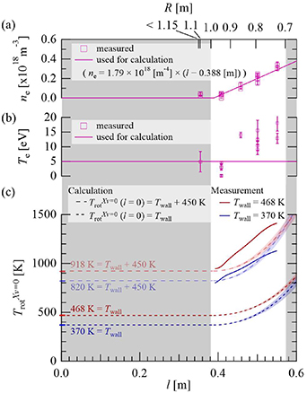
Figure 12. Measurement and calculation results in QUEST. (a)  , (b)
, (b)  , and (c)
  plotted versus (top)
  and (bottom)
  . Markers in (a) and (b) show the values measured by Thomson scattering for both
  conditions. Lines show the profiles used for the calculation. (c) Comparison of measured and calculated
  . Lines in red correspond to the calculation or measurement results for the higher
  , and those in blue correspond to the results for the lower
  . The solid and dashed lines show the measured
  and that calculated considering only the rotational excitation (Rot). The dashed lines shown in darker and lighter colors represent
  calculated with
  and
and  450 K, respectively. Unshaded region corresponds to
  0.7–1.0 m where
  was evaluated.
Download figure:
Standard image High-resolution imageIn LTX-β,  was measured with different
  and
and  conditions considering temporal evolution of the plasma parameters and external heating of the shells, respectively. The
  -axis is defined as in the radial direction at the same height as chords 4 or 5, with its origin on the high-field-side surface of the shell (see figures 5(b) and 9(a)). As described in section 3.3, the Fulcher-α emission was approximated as a point source at
  0.03 m, and the measured
  is plotted by markers at this position in figure 13(b). Note that
  measured for chords 4 and 5 was analyzed assuming up-down symmetry in the plasma. The
  profile measured with the probe is shown by markers in figure 13(a). The measured
  was higher than
  for all the conditions. The
  dependence of
  is shown in figure 14. For both conditions,
  was evaluated using the model described in section 2. Two types of
  profiles shown by magenta lines in figure 13(a) were used for the calculation. The profiles were approximated to be linear, and the two lines in the figure correspond to the conditions of
  0.03 m
 1017 and 1018 m–3. As done for the QUEST analysis, the profile of
  was approximated to be constant. The values for the other plasma parameters were determined based on those of QUEST because of the similar size of the device and similar values of
  and
and  (see table 3). The calculation was conducted at
  297 and 466 K, the same conditions as the measurements, considering only the rotational excitation (Rot), and the initial values
  were set at
  . The calculation results are shown by the dashed lines in darker colors in figures 13(b) and 14. The calculated
  was smaller than the measurements by 560 K at
  0.03 m. The rotational temperature
  was recalculated with the initial conditions of
  increased by 560 K and the results are plotted by the dashed lines in lighter colors in figures 13(b) and 14. Assuming
  500–600 K, the increase in
  with
with  is comparable to the calculated
  . The discrepancy of 500–600 K is presumably produced by the surface recombination and is nearly equal to the value obtained in QUEST, whose plasma-facing walls made of a different material from that of LTX-β as shown in table 3. For more precise examination, measurement of the spatial profiles of Fulcher-α emission and
  is required.

Figure 13. Measurement and calculation results in LTX-β. (a) Measured and interpolated  versus
  . Markers show the
  measured with the probe, and their colors indicate
  conditions. Lines show the profile used for the calculation. (b) Comparison of measured and calculated
  plotted versus
  . Lines and markers in red correspond to the calculation or measurement results for the higher
  , and those in blue correspond to the results for the lower
  . The markers show the measured
  . The dashed lines show
  calculated considering only the rotational excitation. Those in darker and lighter colors represent
  calculated with
  and
and  560 K, respectively. Note that the markers are slightly shifted left and right to avoid overlap each other.
Download figure:
Standard image High-resolution image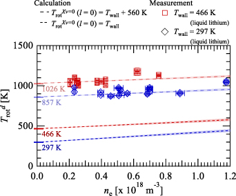
Figure 14. Comparison of measured and calculated  at
at  0.03 m plotted versus
  in LTX-β. Lines and markers in red correspond to the calculation or measurement results for the higher
  , and those in blue correspond to the results for the lower
  . The measured
  is represented by markers and plotted versus
  measured with the probe. Dashed lines show
  calculated considering only the rotational excitation, and those in darker and lighter colors represent
  calculated with
  and
and  560 K, respectively.
Download figure:
Standard image High-resolution imageIn DIII-D,  was measured with different
  ,
,  , and
, and  in attached L-mode plasmas. The
  -axis was defined as an axis perpendicular to the divertor target as illustrated in figures 5(c) and 10(a). In the case of DIII-D, the value of
  is equal to the vertical distance from the divertor target. As described in section 3.3, the Fulcher-α emission was approximated as a point source at
  0.01 m, and the measured
  is plotted by crosses at this position in figure 15(a). The measured
  was higher than
  for all the conditions, and the differences between the measured
  and
and  are the largest in the three tokamaks. For a density of 9
  1018–6
  1019, an increase in
  of ∼1000 K was observed. The collisional-radiative increase
  was calculated and compared to the measurement results. The profiles of
  and
and  were assumed to be constant where the emission is localized, and their values were determined from those measured by Thomson scattering. The values of
  were set at multiplies of 5 eV because of the small dependence of the calculation results on them as described in section 2.2. For the other parameters, their values were inferred from the results of the EDGE2-EIRENE edge fluid code simulations [32] for a hydrogen plasma and are summarized in table 3. The calculation was conducted at the same
  conditions as the measurements, and
  was set at
  . The calculation results are shown by dashed and chain lines in figure 15. The shading in figure 15(a) shows the uncertainty coming from the
  uncertainty, and the values are also shown in the legend. These results are also plotted versus
  in figure 15(b). Note that the calculation result considering all the processes (wEle) is removed for
  478 K because of a large uncertainty due to the ignorance of processes changing the nuclear spin of hydrogen molecules (see the supplementary data). The calculated
  is ∼1000 K at
  0.01 m and larger than those for the other two tokamaks owing to the larger
  . This is consistent with the larger differences in the measured
  from
from  . The calculated
  matches the measured increase within a factor of three. This larger difference between the calculation and measurement results may be attributed to the uncertainty of the position of the point emission because of the limited spatial resolution of the Tangential TV diagnostics (
 0.01 m). Additionally, the difference may become smaller by considering spatial profiles of the Fulcher-α emission and
  . The increase in
  with
with  was not observed in DIII-D, but the dependence may appear when the evaluation of
  is improved. The
  dependence of
  derived from the calculation was consistent with that previously obtained for deuterium discharges in DIII-D [5]. In the previous study,
  was measured by Thomson scattering, and the Fulcher-α emission was measured using a viewing chord directed to the outer strike point. As shown in figure 2, the measured
  dependence (markers) agreed with the derived relation (purple line) when using
  2 mm. The distance of 2 mm, while adjusted here to match the measurements, is comparable to the location of the emission evaluated from the Tangential TV diagnostics, considering its spatial resolution is approximately 0.01 m.

Figure 15. Comparison of measured (markers) and calculated (lines)  plotted versus (a)
  and (b)
  measured by Thomson scattering in DIII-D. The short dashed, chain, long dashed lines show the calculated
  considering only the rotational (Rot), rovibrational (wVib), and electronic (wEle) excitation and deexcitation processes, respectively, by both electron and proton collisions (see table 2). The measurement results in D2 plasma [5] is also shown in (b). The inset in (b) is the expanded view.
Download figure:
Standard image High-resolution imageThe increases,  and
and  , were evaluated from difference between
  and
and  measured in the three tokamaks. The difference is plotted versus integral of
  with respect to
  (
( ) in figure 16. The integral
  is derived using the same
  profile as that used to calculate
  . The measured difference
  increased with
  , and had a similar dependence on
  as calculated
  except for that measured in DIII-D, whose
  has a large uncertainty originating from the uncertainty of the position of the Fulcher-α emission. This indicates that
  depends on
  , i.e. the travel history of molecules and can be independent from
  and surface material. The difference between
  and calculated
  may reflect
  . However,
  can be affected by the molecules moving toward and colliding with the wall, which are ignored in the model. The measurement of fluxes of hydrogen ion, atom, and molecules requires to evaluate the effect and
  .
.

Figure 16. Difference between  and
and  plotted versus integral of
  with respect to
  . Solid lines, squares and diamonds, and crosses are that measured in QUEST, LTX-β, and DIII-D. Colors of lines and markers are same as those in figures 12–15. Gray dashed line shows increase due to collisional-radiative processes (
 ) calculated for
  500 K and
  10 eV.
Download figure:
Standard image High-resolution image
4. Conclusion
In this work, the rotational temperature of hydrogen molecules  was measured, and the increase in
  with
with  and that by collisional-radiative processes in the plasma were evaluated. Previous research implies that
  of the desorbed molecules is affected by surface effects (surface temperature
  and excitation due to recombination
  ) and by collisional-radiative processes in the plasma (
 ). The latter was modeled using rate equations considering an extensive set of collisional-radiative processes, i.e. electron and proton collisional excitation and deexcitation and spontaneous emission. The calculation results revealed the high sensitivity of
  and
and  for the increase in
  though the effects of
  ,
,  , and
, and  were negligible. The relative effects of the rotational, rovibrational, and rovibronic excitation and deexcitation processes were evaluated, and it was found that the latter two processes affect when the product of the density and
  is higher than 1017 m–2. The Fulcher-α emission lines of hydrogen molecules (600–608 nm) were measured to estimate
  in three tokamaks with different plasma-facing materials: QUEST (APS-W), LTX-β (solid and liquid lithium), and DIII-D (ATJ graphite). The rotational temperature for the d state
  was derived from the relative intensity of the measured spectra, and
  was estimated. In QUEST, increases in
  with
with  and
and  were observed, and the measurement results agree well with the calculated profile when assuming
  450 K. These results suggest that the collisional-radiative processes cause the increases in
  in the plasma and
  near the plasma-facing wall depends on
  . In LTX-β, increases in
  with
with  and
and  were observed, and the measurement results agree with the calculated profile when assuming
  500–600 K. In DIII-D,
  was measured with higher
  conditions than the other tokamaks. The measured increase in
  is consistent with the calculation results within a factor of three, which indicates the increase by the collisional-radiative processes in plasma with higher
  . However, the spatial resolution for localization of the H2 emission is poor and requires further improvement in the future. The calculated
  was also consistent with
  dependence of
  previously measured for deuterium discharges in DIII-D [5]. The increases in
  ,
,  and
and  , were evaluated from
  measured in the three tokamaks. The difference
  increased with
  and had a similar dependence on
  except for that obtained in DIII-D. This suggests that
  depends on the travel history of molecules and can be independent from
  and surface material for the parameters described in this paper. The evaluation of
  requires the measurement of fluxes of hydrogen ion, atom, and molecules, since the difference
  may be affected by the molecules moving toward and colliding with the wall. These results show that
  of the desorbed molecules are affected by
  and collisional-radiative processes. This indicates that the increase in
  can be estimated from measured
  and
and  evaluated using the model.
Acknowledgments
The first author is supported by Mori Manufacturing Research and Technology Foundation. The authors thank M. Ono for supporting the experiment in LTX-β, and T. Abrams for supporting the experiment in DIII-D. The authors are grateful to M. Čížek for providing the cross section data. The authors would like to thank the staff members of the machine shop of Kyoto University for their help with the fabrication of the spectroscopic system used in QUEST. This work was supported by bilateral collaboration programs of NIFS (NIFS19KUTR140, NIFS20KUTR156), Japan/U. S. Cooperation in Fusion Research and Development, and USDoE under contracts DE-AC52-07NA27344 (LLNL), DE-AC02-09CH11466 (Princeton University) and DE-AC05-00OR22725 (ORNL). This material is based upon work supported by the US. Department of Energy, Office of Science, Office of Fusion Energy Sciences, using the DIII-D National Fusion Facility, a DOE Office of Science user facility, under Award(s) DE-FC02-04ER54698.
Disclaimer
This report was prepared as an account of work sponsored by an agency of the United States Government. Neither the United States Government nor any agency thereof, nor any of their employees, makes any warranty, express or implied, or assumes any legal liability or responsibility for the accuracy, completeness, or usefulness of any information, apparatus, product, or process disclosed, or represents that its use would not infringe privately owned rights. Reference herein to any specific commercial product, process, or service by trade name, trademark, manufacturer, or otherwise does not necessarily constitute or imply its endorsement, recommendation, or favoring by the United States Government or any agency thereof. The views and opinions of authors expressed herein do not necessarily state or reflect those of the United States Government or any agency thereof.
Supplementary data (0.5 MB PDF)