


Abstract
Fuel retention in plasma facing tungsten components is a critical phenomenon affecting the mechanical integrity and radiological safety of fusion reactors. It is known that hydrogen can become trapped in small defect clusters, internal surfaces, dislocations, and/or impurities, and so it is common practice to seed W subsurfaces with irradiation defects in an attempt to precondition the system to absorb hydrogen. The amount of H can later be tallied by performing careful thermal desorption tests where released temperature peaks are mapped to specific binding energies of hydrogen to defect clusters and/or microstructural features of the material. While this provides useful information about the potential trapping processes, modeling can play an important role in elucidating the detailed microscopic mechanisms that lead to hydrogen retention in damaged tungsten. In this paper, we develop a detailed kinetic model of hydrogen penetration and trapping inspired by recent experiments combining ion irradiation, hydrogen plasma exposure, and thermal desorption. We use the stochastic cluster dynamics method to solve the system of coupled partial differential equations representing the mean field description of the multispecies system. The model resolves the spatial distribution of defects and hydrogen clusters during the three processes carried out experimentally and is parameterized with information from atomistic calculations. We find that the calculated thermal desorption spectra are broadly characterized by three H emission regions: (i) a low temperature one where dislocations are the main contributors to the release peaks; (ii) an intermediate one governed by hydrogen release from small overpressurized clusters with multiple overlapping peaks, and (iii) a high temperature one defined by clean isolated emission peaks from large underpressurized bubbles. These three temperature intervals are seen to largely correlate with the depth at which the clusters are found. The relevance of the 'super abundant' vacancy mechanism is assessed, finding that its main role is to transfer more clusters from the intermediate to the high temperature regions as its relevance increases. We find this picture to be in very good agreement with the experiments, adding confidence to the predictive potential of the models and their useto understand irradiation damage and plasma exposure effects in plasma facing components.
Export citation and abstract BibTeX RIS
1. Introduction
Tungsten (W) is being considered as a candidate plasma facing material (PFM) in magnetic fusion energy devices due, among others, to its high strength, high thermal conductivity, and low erosion susceptibility. Although W lacks the formation of stable hydrides, tritium fluxes as high as 1024 m−2s−1 are expected on the DEMO5 divertor [1, 2], potentially leading to severe surface blistering [3–7], cracking [8], hydrogen embrittlement [9, 10], as well as creating safety and waste disposal concerns [11]. Retention of tritium (T), deuterium (D), or hydrogen (H) in as-fabricated W specimens is highly dependent on synthesis, thermal history, and intrinsic microstructure [12–16]. Understanding T/D/H retention in plasma-facing components is critical, as the viability of a D-T fusion energy source relies on the ability to breed sufficient T fuel for self-sustaining operation. For this, the allowable T retention probability limit must be very low (below ∼ 10−6) in the first wall and PFM's to achieve a tritium breeding ratio larger than unity [17]. Since the equilibrium vacancy concentration in the 500∼ 900 K temperature range is no higher than 10−9, thermal retention of hydrogen is generally considered negligible [18, 19]. However, displacement damage at the level of 0.01 to 0.1 dpa introduced by energetic particle irradiation is known to lead to a significant (tenfold or more) increase in fuel retention [20, 21], making T inventory control more challenging during reactor operation subjected to neutron exposure. It is believed that defect clusters from irradiation can trap hydrogen atoms and contribute to the increase of fuel retention in the material. Moreover, it is assumed that these clusters are primarily vacancy-hydrogen complexes (onwards referred to as VmHn defects containing m vacancies and n hydrogen atoms). Understanding the interplay between irradiation damage and T/D/H retention is thus of paramount importance to understand materials degradation and response, and to improve thermo-mechanical engineering and design.
Lack of suitable neutron sources has spurred the use of heavy ions as surrogates of neutron damage to study materials degradation under fusion conditions. Despite wide differences in dose rate and spatial penetration, heavy ions have been proven an effective means to seed irradiation defects in materials subsequently exposed to hydrogen plasmas [22]. The amount of hydrogen trapped and the nature of the defect clusters present in the material is generally assessed a posteriori by thermal desorption spectroscopy (TDS), correlating hydrogen release with temperature to quantify detrapping energies of hydrogen from clusters [23–33]. TDS is an integrated measurement in the sense that it does not provide spatial information about the distribution and size of VmHn clusters. Insight into such properties of the defect cluster population can currently be gained from techniques such as electron microscopy (TEM) or nuclear reaction analysis (NRA) [34–38]. As well, x-ray diffuse scattering can provide information about the nature and size of the defects [39]. In all, the study of hydrogen retention in PFM's requires a multidimensional experimental effort involving heavy-particle irradiation, hydrogen plasma exposure, thermal desorption, and cross-characterization of defect populations and quantitative analysis of de-trapping energies using multiple techniques.
Given the inherent complexities discussed above, modeling has emerged as an effective option to contribute to our understanding of the fuel retention process at multiple levels. Kinetic transport methods such as rate theory (RT) or kinetic Monte Carlo (kMC) are natural choices to simulate the long-term kinetics of H penetration and trapping at length scales that capture surface and subsurface regions. As such, these methods must possess spatial resolution. While trivial for kMC calculations, this implies solving a system of partial differential equations (PDEs) formulated under the mean-field approximation for RT models6. This technique has been widely used to simulate H effects on W surfaces, partially owing to drastic advances in our capability to use first-principles atomistic methods based either on semi-empirical potentials—as in molecular dynamics (MD) simulations—or density functional theory (DFT) to account for the complex energy landscape of H penetration in the material and define the physical coefficients needed for kinetic transport simulations [40, 41]. Indeed, atomistic calculations have provided and continue to provide fundamental kinetic parameters with unprecedented levels of physical accuracy. This includes energies for H adsorption and desorption in W [42], migration energies [43], characterization of the bi-dimensional VmHn dissociation energy map [44–46], as well as—lately—He/H interaction energies [47]. Furthermore, our understanding of hydrogen retention processes has been enriched by consideration of yet-experimentally-unconfirmed physical processes such as the trap mutation or the superabundant vacancy mechanisms [48–50], whose effect can be evaluated and tested using modeling and simulation in order to assess their applicability.
However, both RT and kMC suffer from intrinsic numerical limitations that hinder their application to the current problem. RT calculations cannot capture the full catalog of VmHn species due to the explosive growth in the number of PDEs to be considered for multispecies cases (vacancies, self-interstitials, hydrogen atoms, and clusters thereof) [51–55]. As well, they lack spatial correlations, a direct consequence of the mean-field approximation. For their part, direct kMC simulations are subjected to stiffness due to time scale separation of physical events and slow time evolution [56, 57]. In this work, we carry out spatially-resolved stochastic cluster dynamics (SR-SCD) simulations of a recent set of experiments performed by several of the co-authors involving (i) Cu-ion irradiation of single crystal W coupons, (ii) exposure to low-temperature H plasmas, and (iii) thermal desorption spectroscopy analysis [58, 61].
The paper is organized as follows. A brief description of the experimental measurements is provided in section 2. Details of SR-SCD model, including underlying theory, the physical processes considered, and the parameterization employed are given in sections 3 and 4. This is followed by the results in section 5 and a brief technical discussion in section 6. We end with the conclusions and the acknowledgments.
2. Experimental details and analysis
To avoid activated PFM samples, the experiments use deuterium and heavy ions as proxies for tritium and fusion neutrons, respectively. The tungsten samples, with dimensions of 6.0 and 1.5 mm in diameter and thickness, were made of 99.95 wt% powder metallurgy polycrystalline W rod. The samples were then delivered to the Ion Beam Materials Laboratory (IBML) at Los Alamos National Laboratory for Cu-ion irradiation, then transported back to UCSD for D2 plasma exposure at the PISCES-E facility. After plasma exposure, the samples were cooled in air down to room temperature and later analyzed using thermal desorption spectroscopy at the PISCES laboratory. A brief explanation and timeline of each one of the experimental stages follows:
- (a)The tungsten specimens were dynamically annealed (stage III relaxation, i.e. monovacancy motion, in single crystal tungsten takes place at approximately 600 K) [59, 60]), each at a fixed temperature ranging from 300 to 1243 K (which is the expected temperature interval of PFM in ITER or DEMO), while irradiated with 3.4-MeV Cu ions to a dose of 1.82 × 10¹⁸ ions per m2 (1 dpa ≈ 9.1 × 10¹⁸ ions per m2).
- (b)Approximately two weeks later, the irradiated specimens were exposed to D2 plasmas up to a fluence of 1024 D m−2. During D2 exposure, samples were held to 383 K and biased by implantation of 110-eV D ions.
- (c)The plasma facing surfaces of samples were mechanically polished to mirror finish. The surface remained untarnished and no observable color change was noted on the exposed surface either after plasma treatment or prior to TDS. While this batch of samples was not analyzed for oxide formation, other W samples exposed to D plasma have shown minimal oxide formation from exposure to air at room temperature. While the thin oxide layer that forms does so almost immediately, plasma bombardment cleans the native oxides from the surface early during the plasma exposure process [62], so that the exposed surface is clean, although the oxide unavoidably remains during TDS.
- (d)The samples were cooled at ambient conditions from the plasma exposure temperature of 383 K down to room temperature (which takes approximately five minutes) prior to thermal desorption, and subsequently exposed to atmosphere for two weeks prior to Nuclear Reaction Analysis (NRA) performed at IBML.
- (e)Finally, the samples were transported back to UCSD and, after approximately one more week, were thermally desorbed in the PISCES laboratory .
Nuclear reaction analysis and thermal desorption spectroscopy measured the spatial D concentration profile and temperature dependent D release, respectively. The NRA-measured D profile correlated well with the defect profile calculated using SRIM. Total D retention measured by both NRA and TDS show a significant reduction with increased dynamic annealing temperature, approaching intrinsic D retention values when annealed at 1243 K. Detailed information about the experimental procedure and measurements can be found in reference [58]. For the purposes of the modeling, we use H ions instead of deuterons, under the assumption that their chemo-physical behavior is equivalent under non-inertial conditions.
3. Theory and methods
Quantifying hydrogen transport and accumulation in plasma-exposed W necessitates understanding the pertinent energy landscape that H atoms encounter. Figure 1 shows a schematic diagram7 of the near-surface region of the PFM divided into three zones: the 'vacuum', representing the plasma boundary region, the 'surface', representing the first few nanometers where material properties are significantly affected by their proximity to the material's edge, and the 'bulk', where hydrogen atoms do not feel the effect of the surface. The figure illustrates the rich variety of energy barriers experienced by hydrogen as it penetrates the solid from the plasma region. The definitions of the energy parameters shown in the figure are provided in table 1. As additional clarification, Er is analogous to Em but defined only for the surface region.  and Es represent the energy barriers for an H atom to escape the surface (Es out towards the vacuum, and
  towards the bulk). These two energies are a manifestation of the fact that the material surface has a high affinity for H atoms (a process akin to passivation).
  determines the solubility of H in W at each temperature, which gives the equilibrium concentration of dissolved hydrogen. Each energy depicted in figure 1 represents a kinetic process defined by an event rate. These rates control the time evolution of H in the system. As such, every one of these parameters must be obtained using a first-principles method (typically electronic structure calculations or semi-empirical potentials). We discuss this starting in section 3.3.

Figure 1. Schematic diagram of the energy landscape for H penetration and trapping in tungsten. All energy barriers are defined in table 1. Deep traps in the bulk region (shaded green) correspond to accumulation of H atoms at vacancy-hydrogen clusters. Reproduced courtesy of IAEA. Figure adapted from [42]. © EURATOM 2017.
Download figure:
Standard image High-resolution imageTable 1. Description of energy barriers for the energy landscape shown in figure 1.
| Symbol | Description |
|---|---|
 |
energy cost of the H H+H dissociation reaction in vacuum H+H dissociation reaction in vacuum |
 |
barrier to penetrate of an H atom into the bulk |
| Es | H surface desorption barrier |
 |
heat of solution of H in bulk W |
| Em | migration energy of H atoms in bulk W |
| Er | diffusion barrier from the bulk to the surface region |
| Eb | H trapping energies at defects in W |
3.1. Stochastic cluster dynamics model with spatial resolution
Here we use the extension of the stochastic cluster dynamics method (SCD) [63] to perform all simulations. SCD is a stochastic variant of the mean-field rate theory technique, alternative to the standard implementations based on ordinary differential equation (ODE) systems, that eliminates the need to solve exceedingly large sets of equations and relies instead on sparse stochastic sampling from the underlying kinetic master equation. Rather than dealing with continuously varying defect concentrations Ci, SCD evolves integer-valued defect populations Ni in a finite material volume Ω, thus limiting the number of 'active' ODEs at any given moment. Mathematically, SCD recasts the standard ODE system:
into stochastic equations of the form:
where the subindices i, j, and k refer to a given defect species, and q runs over all potential defect sinks. The set  represents the reaction rates of 0th (insertion), 1st (thermal dissociation, annihilation at sinks), and 2nd (binary reactions) order kinetic processes taking place inside Ω, and is obtained directly from the standard coefficients
  as:
as:
The value of Ω chosen must satisfy

where  is the maximum diffusion length li of any species i in the system, defined as:

Here, Di and Ri are the diffusivity and the lifetime of a mobile species within Ω. The above expression is akin to the stability criterion in explicit finite difference models. From equation (2),  . The system of equations (2) is then solved using the kinetic Monte Carlo (residence-time) algorithm by sampling from the set
  with the correct probability and executing the selected events. Details of the microstructure such as dislocation densities and grain size are captured within SCD in the mean-field sense, i.e. in the form of effective sink strengths for hydrogen atoms. For example, the value of siq in equation (1) for dislocation and grain boundary defect sinks is:
where  is the dislocation density and d is the grain size (in this case, q = 1 ≡ 'd' and q = 2 ≡ 'gb').
SCD has been applied in a variety of scenarios not involving concentration gradients [63, 64]. However, equation (1) must be expanded into a transport equation (i.e. a partial differential equation, or PDE) by adding a Fickian term of the type:
where Di is the diffusivity of species i, and  is used for simplicity to represent all of the terms in the r.h.s. of equation (1). To cast equation (6) into a stochastic form, the transport term must be converted to a reaction rate in the finite volume Ω. As several authors have shown, this can be readily done by applying the divergence theorem and approximating the gradient term in terms of the numbers of species in neighboring elements [52, 65]. In the most general 3D case:
where α is a subindex that represents the current element, and β represents the neighboring elements (β = 1, ..., 6 in 3D).  is the dividing surface between neighboring elements α and β,
  is the distance between their centers, and
  is the current element's volume. Figure 2 shows a schematic diagram of the geometry of two generic volume elements. In this fashion, each term of the above sum represents the rate of migration of species i from volume element α to β, which can be now added to the r.h.s. of equation (2) and sampled stochastically as any other event using the residence-time algorithm.
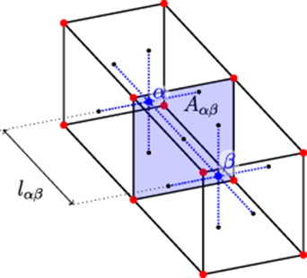
Figure 2. Schematic diagram of two volume elements of a 3D space discretization used to calculate spatial gradients within SCD.
Download figure:
Standard image High-resolution imageThe extension of equation (2) from an ODE system into a PDE system can be written for species i in volume element m as:
For regular cubic meshes, or in 1D, the Fickian term simply reduces to  , where l is the element size. This is the approach employed here.
3.2. Source term and determination of coefficients gi
As described by Marian and Bulatov [63], SCD is ideally suited to deal with the probabilistic aspects of irradiation damage. Once a suitable source function is constructed, one can accurately sample it to create defect distributions. Establishing the source term requires the calculation of recoil energy distributions as a function of depth to be used in SR-SCD calculations. Primary damage is generated from a W-recoil distribution obtained using the SRIM software package [66] for approximately 1000 Cu ions with the same incident energy of 3.4 MeV. According to the calculations, only about 43.5% or 1.48 MeV of the total incident energy is expended on lattice damage, with the rest lost on ionization via electronic stopping. We call this energy ED. The recoil spectra are given as cumulative distribution functions  , seen in figure 3 as a function of target depth. The average PKA energy from this distribution comes out to be
  keV. These functions are then used to obtain random samples of the primary knock-on atom (PKA) energies
  by solving
  , where ξ is a random number uniformly distributed in (0, 1]. Note that
  , where P(E) is the normalized recoil energy spectrum.

Figure 3. Cumulative Cu recoil distribution obtained from SRIM for 3.4-MeV ion irradiations of W surfaces as a function of target depth. The area contained by the dashed line—representing the cumulative value of in each depth bin—amounts to unity to maintain the cumulative probabilistic nature of C(E). The dashed line also represents the damage function γ in equation (8), which peaks with a value of 1.2 × 10⁻³ displacements per ion per micron at a depth of approximately 0.9 µm.
Download figure:
Standard image High-resolution imageThe rate of Cu-ion insertion is calculated as:

where φ is the ion flux, ρa is the atomic density of W, and γ is a damage function calculated within SRIM and measured in units of displacements per ion per unit length, and corresponds to the dashed line shown in figure 3. Once an ion impact event is selected in the simulation volume, a sequence of PKA energies is obtained following the procedure just described until the sum of all sampled recoil energies reaches ED. The insertion coefficients g are obtained by sampling from discrete distributions parameterized to reproduce sub-cascade statistics collected from hundreds of MD cascade simulations at different temperatures [67, 68]. Specifically, the number of Frenkel pairs produced as a function of PKA energy are:
where  is given in eV. The dependence of NF with temperature was seen to be weak and is not considered in this study. We set the minimum value of
  to produce a stable Frenkel pair inside the material to be 620 eV [64]. For their part, the fractions of clustered SIAs and vacancies
  ,
,  depend strongly on, respectively, PKA energy and temperature [69]:


where  is the absolute irradiation temperature.
3.3. Defect dissociation reactions, sink-induced absorption and emission.
The sij coefficients used in equation (7) dictate the propensity of a species i to be absorbed at a sink of type j. Generally, these sinks are intrinsic microstructural heterogeneities, such as grain boundaries (GBs), precipitates, free surfaces, and/or dislocations (refer to equation (5)). In the present study, we consider pure W single crystal surfaces, which eliminates the first two types of sinks. Also, since the surface of the material is explicitly resolved spatially, one need not to consider free surfaces as independent sinks (the simulations themselves capture the migration of defects to the surface layer). This leaves dislocations as the only microstructural feature that can absorb defects. Sinks are characterized by their sink strength, which for dislocations is directly the dislocation density ρd. The absorption rate of mobile defects i by dislocations is then:

where zi is an appropriate bias factor that captures the increased propensity of some defects over others to be absorbed by dislocations (e.g. SIAs vs. vacancies). Consequently, the number of defects absorbed is simply:

where the superscript 'd' is used to indicate that particular fraction of defects is trapped at the dislocation.
While the absorption of mobile defects and H atoms by dislocations is spontaneous, the inverse process—i.e. emission—is thermally activated with a dissociation energy of Ed (for H atoms, it is ≈ 0.6 eV according to several estimates [70])). After Friedel [71], this emission rate can be expressed as:
The first term (in parentheses) on the r.h.s. of the above expression is a geometric factor that gives the number of possible emission sites from a cylindrical 'tube' around dislocation segments, with a0 the lattice parameter and  . ν0 is an attempt frequency (e.g. the Debye frequency of the material), and
  is the equilibrium concentration of species i. Assuming thermal equilibrium,

where  is the formation energy (for H atoms, this is equivalent to the heat of solution) of species i. In practice, emission from dislocations is only enabled for H atoms, such that—after inserting the expression for
  into equation (13)– the emission rate becomes:
For their part, the dissociation coefficients of VmHn clusters are calculated assuming thermal emission of monomers (H or V) as:
where  are appropriate binding energies of monovacancies or H atoms to a cluster i, and
  are the corresponding migration barriers of vacancies or H atoms in the bulk. ri represents the size of the cluster, typically calculated by assuming a spherical vacancy cluster shape:
with m the number of vacancies in the VmHn cluster and Ωv the vacancy formation volume.
3.4. The 'super-abundant' vacancy model.
Broadly speaking, the super abundant vacancy (SAV) mechanism is a process by which hydrogen assists in the generation of vacancies in a material. Numerous examples of the SAV effect exist in metals, e.g. Ni, Cr, Pd, Al, Mo, or Nb [72–75]. At the atomistic level, the fundamental idea is that as vacancies and vacancy clusters capture hydrogen atoms their internal pressure grows up to an unstable point, after which a vacancy-SIA pair is produced with the extra vacancy helping to relieve the pressure (i.e. decrease the H/V ratio) of the cluster, and a SIA emitted into the bulk. In such fashion, the system is in principle able to absorb an indefinite amount of hydrogen, provided that the H/V ratio (n/m) is kept within the stability limits of the equation of state of the clusters. This is akin to the well-known 'trap-mutation' mechanism observed in W exposed to He plasmas [76]. For hydrogen in tungsten, several authors have introduced this mechanism and discussed the energetics of the process to determine the vacancy-to-hydrogen ratios that trigger the reaction [77–79]. When the energetics of the reaction are favorable, the sequence goes as follows:

such that the ratio changes from  to
to  and a SIA is inserted into the lattice. The stability of the reaction can be assessed in terms of the energies of each of the reactants and products:

such that reaction (16) will take place when the excess energy

becomes negative. These formation energies can be calculated as:
where  is the binding energy between a pure H aggregate with n atoms and a Vm vacancy cluster, and
  is the cohesive energy (eV/atom) of W.
  ,
,  , and
, and  are the heat of solution of H in W, and the vacancy and self-interstitial atom formation energies, respectively. Values for the required binding energies are given in appendix
  eV [80],
  eV [81],
  eV [82], and
  eV [83].
Figure 4 shows a color map of  . The white solid line marks the limit of stability of the SAV mechanism. Above it, reaction (16) becomes energetically favorable and the SAV mechanism becomes active, while, below it, VmHn clusters are stable. This criterion guides the behavior of the clusters and is an independent source of growth during the simulations. This solid line can be approximated by a linear relation whose slope yields the critical x = n/m ratio. For our model, this is equal to x = 4.0, represented as a white dashed line in the figure. However, while figure 4 indicates the thermodynamic stability region of the SAV mechanism, its occurrence may also be controlled by a kinetic barrier (in the manner of standard chemical reactions). Such an energy, which we term
  , defines a transition rate that is enabled only when
  :
:
At present, there are no experimental or numerical estimates of  , and it thus must be obtained through other means. We will return to this point when we discuss the model results below.

Figure 4. Color map of excess energies according to equation (18). The white solid line marks the limit of stability of the SAV mechanism. Above it, reaction (16) becomes energetically favorable and the SAV mechanism is in operation. Below it, VmHn clusters are stable. The dashed line represents a linear fit yielding the optimum hydrogen-to-vacancy ratio.
Download figure:
Standard image High-resolution image4. Model parameterization
4.1. Simulation conditions
Table 2 gives all the numerical parameters and simulation conditions in accordance with the three experimental phases discussed in section 2.
Table 2. Material and simulation parameters employed in the simulations.
| W material parameters: | Symbol | Value | Units | |||
|---|---|---|---|---|---|---|
| Atomic density | ρa | 6.31 × 1028 | ![$[\mathrm{m^{-3}}]$](https://content.cld.iop.org/journals/0029-5515/60/9/096003/revision2/nfab9b3cieqn50.gif) | |||
| Lattice parameter | a0 | 3.16 | Å | |||
| Dislocation density | ρd | 1010 | ![$[\mathrm{m^{-2}}]$](https://content.cld.iop.org/journals/0029-5515/60/9/096003/revision2/nfab9b3cieqn51.gif) | |||
| Cu irradiation parameters: | ||||||
| Irradiation temperatures |  |
300, | 573, | 873, 1023, | 1243 | [K] |
| Ion flux | φ | 1.34 × 10¹⁵ | ![$[\mathrm{m^{-2}s^{-1}}]$](https://content.cld.iop.org/journals/0029-5515/60/9/096003/revision2/nfab9b3cieqn53.gif) | |||
| Ion energy |  |
3.4 | [MeV] | |||
| Dose | (φt) | 0.2 | [dpa] | |||
| H plasma exposure parameters: | ||||||
| Temperature | - | 383 | [K] | |||
| Flux |  |
4.0 × 10²⁰ | ![$[\mathrm{m^{-2}s^{-1}}]$](https://content.cld.iop.org/journals/0029-5515/60/9/096003/revision2/nfab9b3cieqn56.gif) | |||
| Time duration | Δt | 2500 | s | |||
| Deposition energy |  |
113 | ![$[\mathrm{eV}]$](https://content.cld.iop.org/journals/0029-5515/60/9/096003/revision2/nfab9b3cieqn58.gif) | |||
| Thermal desorption parameters: | ||||||
| Heating rate | β | 0.5 | [K·  ] ] | |||
| Temperature range | ΔT | 300 ∼ 1300 | [K] | |||
| Numerical parameters: | ||||||
| Number of spatial elements | n | 101 | - | |||
| Element volume | Ωi | 10−23 | [m3] | |||
| Top layer thickness | ls | 0.54 | [nm] | |||
| Element thickness | li | 20 | [nm] |
4.2. Defect and hydrogen atom energetics in W
The calculation of the transport energetics of defects and hydrogen atoms in tungsten has attracted a great deal of attention in recent years [43, 80, 84, 84–104]. Based on an extensive literature review, we have selected a set of parameters for the diffusivities and energetics of defects and hydrogen, summarized in tables 3 and 4. The first table gives the values of the diffusivities of all mobile species assuming the standard Arrhenius expression for thermally-activated motion  . Table 4 gives additional values for the parameters used in figure 1.


5. Results
5.1. Cu-ion irradiation
Cu-ion irradiation, described in section 2, to a total dose of 0.2 dpa at 300, 573, 873, 1023, and 1243 K results in the accumulation of point defect and defect clusters in the irradiated specimens. Figure 5(a) shows the concentration of vacancy-type defects8 in the entire specimen as a function of dose calculated with SR-SCD. As the figure shows, the defect concentration experiences an incubation period of rapid increase characterized by a power law with scaling exponent 0.5 (which appears to be independent of temperature), followed by convergence to steady state. This steady state is reached more rapidly at elevated temperature, and its final value is indicative of the point at which vacancy and vacancy cluster production is balanced by absorption at sinks. At 300 K the system has not reached this steady state after 0.2 dpa. The accumulation of vacancy defects is substantial, with concentrations approaching 0.02 at.% at 300 and 573 K. The steady state concentrations roughly decrease linearly with temperature. The buildup of SIA clusters is seen to follow identical qualitative trends as vacancies, although with much lower concentrations.

Figure 5. Vacancy-type defect accumulation in W during Cu-ion irradiation at 300, 573, 873, 1023, and 1243 K, respectively. (a) Integrated defect accumulation as a function of dose. (b) Depth profiles at the end of the ion irradiations. The colored bands represent error bars from numerical fluctuations over five independent SR-SCD runs.
Download figure:
Standard image High-resolution imageThe depth distributions at 0.2 dpa for each temperature are plotted in figure 5(b). Consistent with figure 3, defects are distributed uniformly into the material to a depth of approximately 1.4 microns. These initial vacancies and vacancy clusters become the seeds for the formation of larger hydrogen-trapping VmHn complexes during the plasma exposure phase. The clusters are generally small. Figure 6 shows the cluster size distribution after the irradiation phase, with the largest one being a V6 at 573 K.

Figure 6. Vacancy cluster size distribution in W at the end of Cu-ion irradiation stage.
Download figure:
Standard image High-resolution image5.2. Determination of SAV reaction barrier by mapping to experimental results
Next, we simulate the next two phases, i.e. hydrogen plasma exposure and thermal desorption of all irradiated samples. First, however, as introduced in section 3.4, a key parameter to be defined before entering a complete set of simulations of the H exposure phase is the energy barrier  . In the absence of direct measurements or calculations of
  , here we take a backend approach to ascertain its value: we systematically vary it from zero to 1.5 eV and simulate plasma exposure and thermal desorption for each value. We then compare the simulated TDS to the experimental ones and select the value of
  that produces the best match as evaluated using a least-squares error analysis. As an advance of more results to come, in figure 7 we show results for six different scenarios: 0 (equivalent to a 'spontaneous' SAV mechanism), 0.90, 0.95, 1.00, and 1.20 eV. We also show results for simulations under no SAV mechanism. Our results suggest that the best match is obtained for
  eV, which is the value used hereafter to showcase the hydrogen exposure and thermal desorption phases.
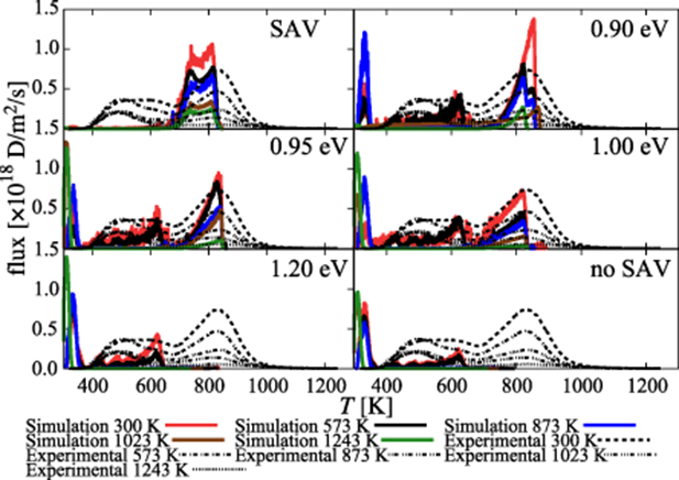
Figure 7. Simulated and experimental hydrogen thermal desorption spectra for the five irradiation temperatures considered in this work under different values of  .
.
Download figure:
Standard image High-resolution image5.3. Hydrogen exposure of irradiated specimens
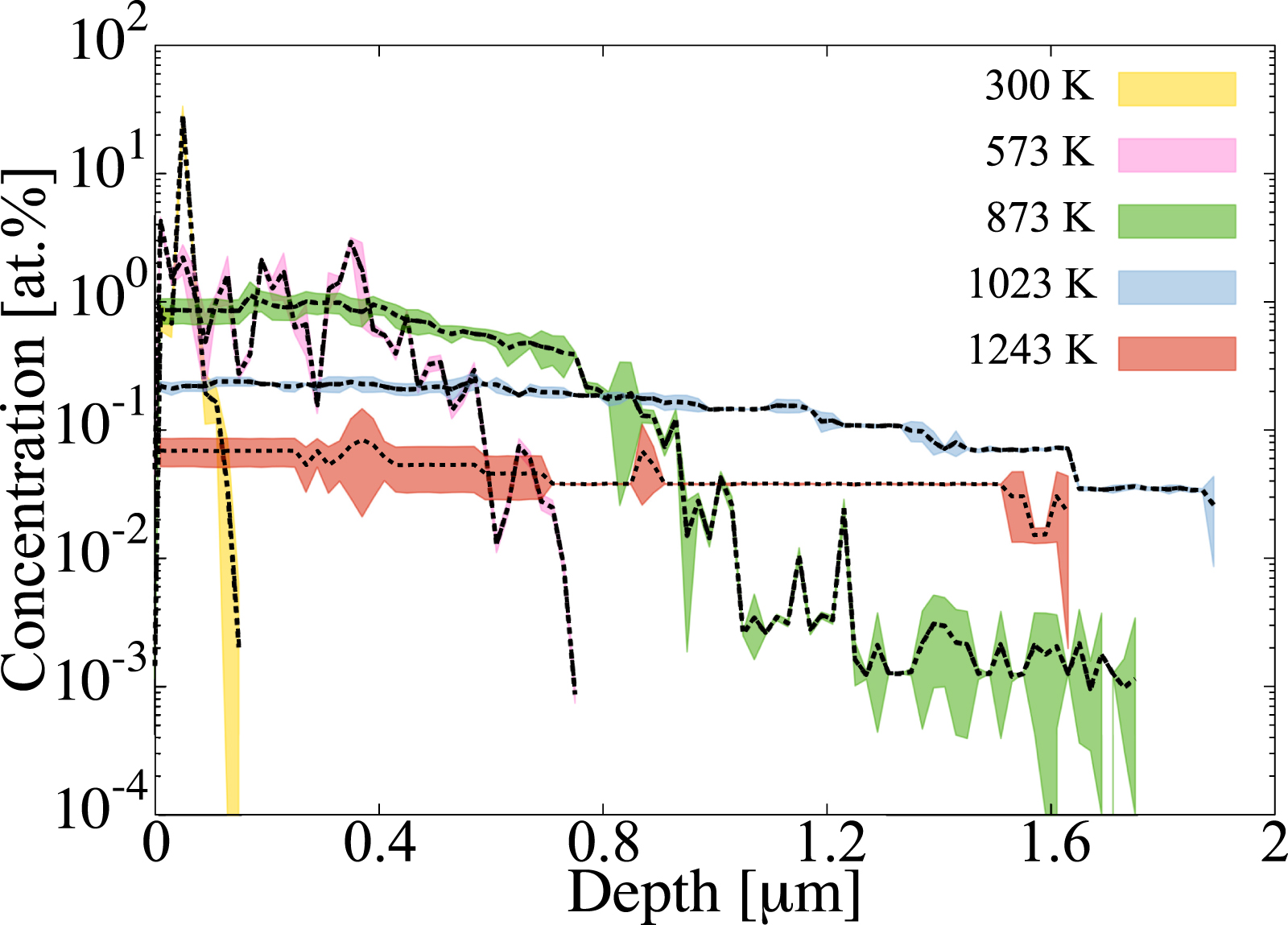
In accordance with experimental conditions, the hydrogen exposure stage is simulated at a temperature of 383 K and a duration 2500 s under a constant hydrogen flux of 4.0 × 10²⁰ m−2s−1 (total fluence 1024 m−2). Figure 8 shows the distribution of hydrogen as a function of depth for each irradiation temperature at the end of the exposure period. Note that the concentrations shown include hydrogen in any form, i.e. free hydrogen monomers as well as H atoms trapped in vacancy clusters. Irradiation temperature is seen to have a noticeable impact on the depth distribution of hydrogen, largely correlated with the distribution of vacancy clusters during the irradiation phase. In general, hydrogen is found deeper, albeit in lower concentrations, the larger  is.
is.

Figure 8. Depth profile of hydrogen in W after 2500 s of exposure to a flux of  . The hydrogen considered in the graph includes both free hydrogen and hydrogen trapped at vacancy clusters. The colored bands represent error bars from numerical fluctuations over five independent SR-SCD runs.
Download figure:
Standard image High-resolution imageThe analysis of the VmHn populations displayed in figure 8 is critical, as it quantitatively establishes the trapping propensity of the material under the conditions explored here. There are two main aspects of this population that must be further studied. One is the relative partition of hydrogen-to-vacancy ratios, x = n/m within the cluster subpopulation. The other is the absolute size of the clusters, which has implications for both the total amount of H stored in the system and the visibility under the microscope of the defects. Next, we provide a detailed analysis of both of these aspects in an attempt to ascertain the fuel footprint in irradiated single-crystal W surfaces.
5.3.1. Stability of hydrogen-vacancy clusters and distribution of hydrogen-to-vacancy ratios.
Figure 9 shows the integrated concentration of VmHn clusters as a function of x for each irradiation temperature case. In keeping with the limits established in figure 4, a dashed line is drawn at x = 4 to show the relative stability of clusters based on their hydrogen-to-vacancy ratio. Clusters with  are generically deemed to be 'underpressurized', i.e. with a propensity to absorb more hydrogen atoms, while clusters with x > 4 are said to be 'overpressurized', i.e. with propensity to release hydrogen (or, when the SAV mechanism is active, to produce vacancy-SIA pairs). On the basis of this partition, two things can be established about the different
  cases: (i) a higher irradiation temperature leads to preferentially underpressurized clusters, while lower temperatures result in an equipartition between under- and overpressurized bubbles; (ii) the range of x observed is 0 to 9.

Figure 9. Histogram of the integrated concentration of vacancy-hydrogen clusters in terms of their hydrogen-to-vacancy ratio after 2500 s of exposure to a hydrogen flux of  .
.
Download figure:
Standard image High-resolution imageFigure 10 shows the depth distribution of the VmHn clusters in terms of their x value as a function of  at the end of the H-exposure phase. The colored bands around each curve represent error bars from numerical fluctuations over five independent SR-SCD runs. Generally, little correlation is observed between x and the depth at which each cluster type is found. Consistent with figure 8, the main effect of irradiation temperature is to result into deeper VmHn cluster penetration.

Figure 10. Depth distribution of the VmHn clusters after 2500 s of H exposure in terms of their hydrogen-to-vacancy ratio as a function of irradiation temperature. We omit the 1243-K case due to its similarity with the results at 1023 K. The colored bands represent error bars from numerical fluctuations over five independent SR-SCD runs.
Download figure:
Standard image High-resolution imageFinally, it is useful to represent the cluster population not just in terms of their x ratios but also in terms of their absolute m and n numbers. Figure 11 shows three-dimensional plots of VmHn clusters as a function of m, n, and the depth at which they are found. Their concentration is given using the color key as specified in the figure. Each subplot corresponds to a specific irradiation temperature. In a similar manner to the distribution of x ratios, key qualitative differences can be appreciated between the lower and higher temperature cases. At lower temperatures, figures 11(a)–(c), most VmHn clusters are located within the first micron of depth, with m and n covering a large span between V H
H to approximately V
 H
H and relatively high concentrations. By contrast, at 1023 and 1243 K (figure 11(d), the figure for
  K is not shown due to its qualitative and quantitative similarity with the 1023-K case) only clusters composed of more than 5500 vacancies are observed at high depths. These large clusters appear in relatively low concentrations. We can synthesize the information contained in these figures into a global size distribution for the end of the exposure phase. This represent essential information to facilitate comparison with experimental distributions, which are limited on the low end by machine resolution. Our results are shown in figure 12 in the form of temperature-smeared Gaussian distributions, with the raw data shown as a histogram in the background. While the figure clearly shows a bi-modal distribution with a peak within one nanometer sizes and another one centered around 6 nm, the standard resolution limit in microscopy of 0.5-to-1.0 nm may prevent revealing the former in experimental size distributions. Techniques such as x-ray diffuse scattering can achieve sub-nanometer resolutions, thus enabling a better comparison with our results [39]. We discuss this further in section 6.2.

Figure 11. VmHn cluster size distributions as a function of m, n, depth, and irradiation temperature. Cluster concentrations are described by a color key. Dashed vertical lines are projections of each data point on he m-n plane for ease of visualization. We omit the 1243-K case due to its similarity with the results at 1023 K.
Download figure:
Standard image High-resolution image
Figure 12. Vacancy-hydrogen cluster size distributions at the end of the hydrogen exposusre simulations. The raw data shown as a histogram with faint colors in the background..
Download figure:
Standard image High-resolution image5.4. Thermal desorption simulations
Thermal desorption processes are thought to be composed of a series of emission events characterized by Gaussian profiles [105, 106]. These Gaussians are centered at temperatures defined by characteristic binding energies representing specific hydrogen release events. It is therefore useful to decompose the desorption profiles shown in the figure into a set of overlapping Gaussian distributions that coincide with the most dominant peaks (or protuberances) in each TD spectrum. Doing this, however, may involve a certain degree of arbitrariness, as these peaks are not always evident (particularly at high temperatures). In any case, we believe that some clear mappings exist and some consistency among the different curves can be found.
Here we focus on the 0.95-eV case in figure 7. Figure 13 shows the decomposed thermal desorption spectra for each irradiation temperature. In performing each decomposition, Gaussians with like colors are used when they are centered at the same desorption temperature (horizontal axis), regardless of the irradiation temperature case. The width of the Gaussians is temperature dependent and has been adjusted so that the contribution to the TD spectrum from the overlap among them is consistent with the full curve. As such, the 300-K and 573-K temperature case (figure 13(a) and 13(b)) is composed of seven distinct Gaussians, each representing a specific desorption mechanism, centered at, respectively, 333, 425, 485, 527, 574, 623, and 836 K. Two of these are shared with the 873-K case, figure 13(c), which is suggestive of identical H-release mechanisms in these two cases. However, the remaining spectra corresponding to the higher irradiation temperatures are characterized by different peaks, namely 310, 842 K (figure 13(d)).
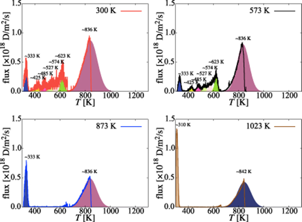
Figure 13. Thermal desorption spectra for each irradiation temperature case decomposed into their constituent Gaussian emission profiles. Each Gaussian is expected to represent a distinct emission mechanism, to be discussed in table 5.
Download figure:
Standard image High-resolution imageTable 5. Operative dissociation mechanisms at each thermal desorption peak temperature for each irradiation temperature. The symbol '⊥' represents 'dislocations'. The simulated dissociation energy,  is obtained as
  . The values for Eb are extracted from table A3 for each specific reaction, while Em comes from table 3. The values for
  were obtained from equation (20).
| T [K] | Irradiation temperature [K] |  [eV] [eV] |  [eV] [eV] | ||||
|---|---|---|---|---|---|---|---|
| 300 | 573 | 873 | 1023 | 1243 | |||
| 310 | – | – | – | ⊥ | ⊥ | 0.85 | 0.70 |
| 333 | ⊥ | ⊥ | ⊥ | – | – | 0.85 | 0.75 |
| 425 | V1H8 →V1H7 | V1H8 → V1H7 | – | – | – | 0.88 | 0.97 |
| 485 | V1H7 → V1H6 | V1H7 → V1H6 | – | – | – | 1.05 | 1.11 |
| V6H23 → V6H22 | – | – | – | 1.06 | |||
| 527 | V1H6 → V1H5 | V1H6 → V1H5 | – | – | – | 1.18 | 1.21 |
| V6H21 → V6H20 | V6H22 → V6H21 | – | – | – | 1.18 | ||
| 574 | V1H5 → V1H3 | V1H5 → V1H3 | – | – | – | 1.28 | 1.32 |
| V6H18 → V6H17 | – | – | – | – | 1.34 | ||
| 623 | V1H3 → V1 | V1H3 → V1 | – | – | – | 1.49 | 1.44 |
| V6H16 → V6H12 | V6H16 → V6H12 | – | – | – | 1.42 | ||
| 836 | V H H → V → V H H |
V H H → V → V H H |
V H H → V → V H H |
– | – | 1.69∼ 1.96 | 1.96 |
| 842 | – | – | – | V H H → V → V H H |
V H H → V → V H H |
1.94∼ 1.96 | 1.97 |
As mentioned above, each one of the Gaussians shown in figure 13 represents a distinct hydrogen emission mechanism. These mechanisms can be directly identified in the simulations from processes defined by equations (14) and (15)), so that we can ascribe a specific dissociation reaction to each emission temperature, Tp. Further, we characterize each Gaussian by a representative dissociation energy  , determined as [107]:
where β is the heating rate. Each  can subsequently be compared with the corresponding dissociation energies corresponding to the specific reactions taking place in the simulations. Those ultimate originate from the data given in table A3. The results of such analyses are provided in table 5.
The information contained in the table is the culmination of the simulation effort of the three-stage experimental study described in section 2. The first column represents all the Gaussian peaks used in figure 13. Columns 2-5 specify the transitions suffered by the clusters during each emission process. With increasing desorption temperature, the emission events include hydrogen emission from dislocations, small overpressurized clusters gradually releasing hydrogen to reduce their hydrogen-to-vacancy ratio towards x = 4, and large underpressurized clusters emitting H atoms until all the hydrogen is evacuated from the system. Finally, the last column lists the corresponding dissociation energies of each dissociation event as calculated with equation (20). We find that, in general, the discrepancy between the  given in table 5 and the actual dissociation energies from table A3 is small. While this simply corroborates that the reactions identified in each temperature interval are consistent with the Gaussian emission peaks, it is an encouraging result that adds confidence to our results.
6. Discussion
The main point of our paper is to test whether one can use fundamental models—combining the most powerful calculations that exist in materials science presently (DFT/electronic structure calculations) with detailed mesoscopic kinetic models than can explore relevant spatiotemporal scales—to understand TDS experiments. We approach the problem from a different angle compared to other studies, with fitting not being a feature of our models by design. Below, we expand on some of the most important findings of this study.
6.1. Physical implications of the present results
Hydrogen thermal desorption in damaged crystals is an extremely complex problem involving numerous processes often co-occurring in a synergistic or non-linear manner. Just listing those considered here gives an idea of this complexity: cascade damage, defect diffusion, hydrogen deposition and penetration, hydrogen passivation, internal hydrogen diffusion, hydrogen absorption and trapping at dislocations and grain boundaries, vacancy cluster-hydrogen reaction, production of vacancies from cluster internal overpressurization, and hydrogen dissociation from clusters, all of it captured with spatiotemporal resolution. The amount of physics needed to undertake simulations of such a challenging process can be staggering, both in terms of the kinetics and thermodynamics of the atomic species involved, as well as in terms of the detailed parameterization needed for physical accuracy and validation. As well, carefully-conducted experiments covering the above processes and in such a way as to facilitate comparison with the models are an invaluable tool to validate and refine the simulations. Fortunately, we believe that the fusion materials community has reached sufficient maturity in all of these fronts to enable the type of study presented here. For example, a systematic effort by researchers to map the energetics of the W-H system using electronic structure calculations and semi-empirical potentials, there are now very reliable data sets available. Thanks to advances in algorithms and computer power, there now exist powerful reaction-diffusion PDE models to study strongly-coupled multispecies problems in great detail. This, combined with several decades of 'know-how' in irradiation damage modeling has open the door to simulations such as those presented here which allow us to push the physical accuracy/computational efficiency tradeoff to unprecedented levels.
In undertaking the present simulation effort, we must also be transparent about two key premises adopted here, namely the presumed infallibility of both experimental results and atomistic calculations. It is beyond the scope of this work to comment in depth about the validity of such premises, and the reader is simply referred to the pertinent sources for details (e.g. references [33, 108] with regard to atomistic calculations, references [44, 58] for the irradiation conditions and plasma exposure, and references [109, 110] for uncertainties in thermal desorption spectroscopy) for details. In general, it is probably safe to say that, as has become common practice in the computational materials science community, both experimental characterization and ab initio calculations have reached a degree of reliability as it relates to PMI studies that allow us to confidently use them in our studies as the 'true' baseline against which to compare model predictions.
With this in mind, the main result of this work is presented in figure 14 (subpanel in figure 7), which we use to discuss the main physical insights gained from the current exercise. Analysis of figures such as those points to two principal features that stand out from within the body of results obtained here:
- (a)Our results conclusively show that, vis-à-vis the experiments, the superabundant vacancy mechanism is a key piece of physics needed to understand the accumulation of vacancy-hydrogen clusters in damaged W subjected to hydrogen exposure point to the existence of a transition barrier. Moreover, we find that the SAV mechanism is accompanied by a transition barrier that modulates changes in the cluster structure. Mapping the simulated TDS to the experimental ones points to a value of 0.95 eV for this transition energy.
- (b)The thermal desorption spectra of H-exposed damaged W surfaces can be broadly decomposed into three distinct emission temperature regions:These temperature regimes are schematically depicted in figure 15, which are in strong qualitatively agreement with the experimental TDS obtained in reference [58].

Figure 14. Thermal desorption spectrum for  .
.
Download figure:
Standard image High-resolution image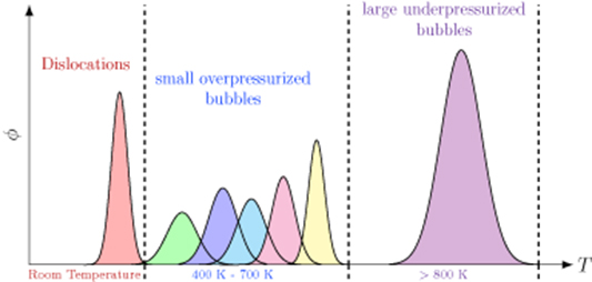
Figure 15. Schematic diagram of the TDS peak distribution. φ represents the desorbed hydrogen flux in arbitrary units.
Download figure:
Standard image High-resolution imageIn this context, the SAV mechanism plays a fundamental role in the final accumulation and release of hydrogen from damaged tungsten surfaces. Going back to figure 7, the absence of a SAV-type mechanism overemphasizes smaller, overpressurized cluster populations, while an unabated9 SAV mechanism leads to an abundance of larger, underpressurized bubbles. In view of these trends, the effect of the SAV activation barrier is clear.  modulates the two extremes (no SAV, spontaneous SAV) and bridges the temperature regions where overpressurized and underpressurized clusters dominate. This is clearly seen in figure 7 and in the experiments, where for
  eV our results show remarkable agreement with both the emission peaks and the emission fluxes measured experimentally.
6.2. Validation
A first attempt at validation of our results can be made by comparing the Sun et al [39] (figure 6 in their paper). At 300 K and 0.2 dpa with 5-MeV Cu ions, the measured vacancy defect concentration was 0.103± 0.02 at. %, while our integrated value from figure 5(b) is 0.023± 0.004 at. %. Part of this 5 × difference is likely attributable to the difference in irradiation energy (5.0 vs 3.4 MeV), although we do not discount other factors related to more fundamental issues such as the model framework. Noteworthy is also the fact that the average cluster sizes in each case (measured vs. simulated) are 10 ± 3 Å and 8.32 ± 0.3 Å, in very close agreement with one another.
Second, related to the experimental effort discussed in section 2, the desorption hydrogen fluence can be measured for each of the irradiation-temperature specimens and compared to the integrated hydrogen release in the simulations. The measurements are shown in figure 16 for two Cu-ion irradiation energies together with the present results. A difference factor of about 2.5 × is observed, which can be partially explained from the analysis of the difference in TDS features that we discuss next.
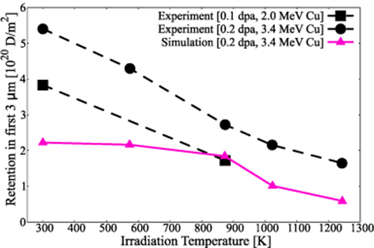
Figure 16. Comparison between experiments and model results of the total hydrogen fluence integrated from the TDS spectra as a function of  . Dashed lines are experimental measurements while the continuous curve represents the model predictions.
Download figure:
Standard image High-resolution imageAnalyses of the experimental peaks between 400 and 700 K (intermediate temperature range) suggests that our simulations underestimate the concentrations of clusters that give rise to the first set of emission peaks (between 400 and 550 K), while they slightly overestimate those in the range between 600 and 700 K. We can specifically point to the reactions that govern each subregime from among those listed in table 5 to analyze this discrepancy. Between 400 and 550 K the peaks are due to the decomposition of V1H7, V1H8, V6H21, and V6H22 clusters. The implication would thus be that the simulations are underestimating these populations relative to the experimental observations. Conversely, between 600 and 700 K the relevant clusters are V1H3, V1H5, V6H16, and V6H18, whose populations would appear to be overestimated in the simulations. This could be due to a number of causes, although given how similar the clusters are in both subregimes, subtle changes in the binding energies would likely suffice to correct this. This is one way simulations such as these can inform the atomistic calculations of the energetics of the W-H system.
Typically, H emission peaks below room temperature are not captured in tungsten in standard TDS experiments. In the few instances where the starting temperature is 300 K or below, experiments have indeed revealed emission of hydrogen and deuterium [111–113]. This is consistent with electronic structure calculations of H trapping energies at edge and screw dislocations ranging between 0.5 and 0.9 eV [70, 114], which would result in desorption peaks below 400 K. Our model includes this latest computational input and, accordingly, it produces a peak at around 300 K. It is worth adding that grain boundaries are predicted to trap hydrogen with energies similar to those of dislocations [ZHOU2011240], such that a contribution to fuel retention from GBs or other two-dimensional defects, if they exist, should not be discounted.
In any case, only dedicated experiments designed for TDS below room temperature can conclusively determine whether the peak exists or not. Results such as those shown here can provide an opportunity for experimental science to verify such low-temperature behavior.
6.3. Role of self-interstitial-type defects
The standard treatment of SIA-type defects in crystalline metals is to assume rapid one-dimensional migration away from the core of displacement cascades towards sinks. When cascades are sufficiently dense from high-energy PKA, dislocation loops can be formed, which, after a critical fluence, may lead to so-called 'rafts' or loop networks. These networks have been shown to be effective hydrogen traps when exposed to a H atmosphere [115].
In the present irradiations, the combination of superficial damage production (the peak dpa occurs at a depth of 0.7 microns) and relatively low PKA energy (≈ 2 keV) results in little SIA-defect accumulation. Additionally, recent DFT calculations have found trapping energies for small H-SIA complexes of around 0.3 eV in W [116, 117]. These energies result in H release in thermal desorption tests at temperatures well below room temperature. For these reasons, we are confident that the SIA-defect contribution to H trapping in the conditions studied in this work can be neglected without much effect on the final results.
When SIA clusters grow to loop sizes, they can become indistinguishable from the dislocation network and trap hydrogen with 0.5∼ 0.9 eV. This of course is already captured in our model, except that the dislocation density is time-invariant. Instances of higher energy PKA over long doses would probably warrant the inclusion of a dislocation density evolution model coupled to the cluster dynamics model to account for loop network formation.
7. Conclusions
The main summary points and conclusions of our paper are:
- (a)We have assembled a simulation methodology based on spatially-resolved stochastic cluster dynamics calculations to simulate a set of experiments involving sequences of ion-irradiations, hydrogen plasma exposure, and hydrogen thermal desorption.
- (b)The models are parameterized using atomistic calculations only (a combination of DFT and semi-empirical potentials) of hydrogen-vacancy cluster energetics. We find that these calculations provide a high degree of numerical accuracy vis-à-vis the experimental results.
- (c)To facilitate comparison, the simulated thermal desorption spectra are analyzed using similar tools to the experiments revealing a set of Gaussian peaks characterizing specific desorption events. In general, these events are different manifestations of the reduction of the hydrogen-to-vacancy ratio from their highest values down to zero. This is achieved by the sequential emission of H monomers at different temperatures, from which the critical binding energies are extracted.
- (d)A principal conclusion of our study is that the thermal desorption spectra are broadly composed of three temperature regions: one below room temperature characterized by emissions from dislocations, and intermediate one characterized by emissions from small overpressurized V-H clusters, and a high temperature one governed by release from large underpressurized bubbles.
- (e)We conclude that the super-abundant vacancy (SAV) formation mechanism (which is equivalent to the so-called 'trap mutation' mechanism in the context of W-He evolution simulations) plays a key role during exposure of tungsten to H plasmas. Under such mechanism, VmHn clusters may absorb H more or less indefinitely provided they can emit self-interstitial atoms. The SAV mechanism acts to shift clusters between the populations belonging to the intermediate and high temperature regimes. We find that a value of 0.95 eV for the SAV activation energy barrier fits the experimental data best.
Acknowledgments
Computer time allocations at UCLA's IDRE Hoffman2 supercomputer are gratefully acknowledged. Useful discussions with the PSI2-Scidac group are recognized. Q. Yu. and J. Marian.'s work was supported by the U.S. Department of Energy's Office of Fusion Energy Sciences (US-DOE), project DE-SC0019157. L. Yang and B. D. Wirth are grateful for partial support from the plasma surface interactions project of the Scientific Discovery through Advanced Computing (SciDAC) program, which is jointly sponsored by the Fusion Energy Sciences (FES) and Advanced Scientific Computing Research (ASCR) programs within the US-DOE Office of Science. M. Simmonds, R. Doerner and G. Tynan's work was supported by the US-DOE under grant DE-FG02-07ER54 912.
: Binding energies of vacancy and hydrogen-vacancy clusters
Table A1. Binding energies of monomers to Iq and Vm clusters used in the simulations. All data from reference [117]. Values for  and
and  are 9.96 [82] and 3.23 eV, respectively [83].
| Species | Eb [eV] |
|---|---|
| I2 | 2.12 |
| I3 | 3.02 |
| I4 | 3.60 |
| I5 | 3.98 |
| I6 | 4.27 |
| I7 | 5.39 |
q  7 7 |
 |
 |
−0.1 |
 |
0.04 |
 |
0.64 |
 |
0.72 |
 |
0.89 |
 |
0.72 |
 |
0.88 |
| m > 8 |  |
Table A2. (Left table) Binding energies of vacancy monomers from VmHn clusters used in this work (from references [44, 45]). The binding energies are given in terms of the H-to-V ratio of the cluster, x = n/m, and include a value for the emission of a vacancy and a different value for the emission of a hydrogen atom (indicated in each case). (Right table) Binding energies of H monomers to SIA-hydrogen clusters (values from reference [44]).
| Eb [eV] | |
|---|---|
| x | V1 |
| 1 | 1.6 |
| 2 | 2.1 |
| 3 | 2.4 |
| 4 | 3.9 |
| 5 | 4.4 |
| 6 | 5.8 |
| 7 | 7.0 |
| 8 | 8.2 |
| 9 | 9.8 |
| 10 | 11.2 |
| 11 | 13.65 |
| 12 | 15.88 |
| 13 | 18.30 |
| 14 | 20.92 |
| 15 | 23.73 |
| Cluster type |  [eV] [eV] |
 |
0.67 |
 |
0.40 |
 |
0.22 |
 |
0.05 |
 |
0.57 |
 |
0.45 |
 |
0.22 |
 |
0.1 |
| IqHn |  |
Table A3. Binding energies of hydrogen monomers from VmHn clusters used in this work (from reference [108]). The binding energies are given in terms of the H-to-V ratio of the cluster, x = n/m, and the cluster size, number of vacancies m. An empirical relation approximating the data was obtained using symbolic regression [118]:  .
.
| Eb [eV] | ||||||||||
|---|---|---|---|---|---|---|---|---|---|---|
 |
1.65 284 | 1.64 638 | 1.64 638 | 1.64 638 | 1.64 638 | 1.64 638 | 1.64 638 | 1.64 638 | ||
| 1 | 1.17 486 | 1.41 062 | 1.39 447 | 1.52 366 | 1.52 366 | 1.52 366 | 1.52 366 | 1.52 366 | 1.52 366 | 1.52 366 |
| 2 | 1.18 455 | 1.37 186 | 1.36 218 | 1.38 478 | 1.38 478 | 1.38 478 | 1.38 478 | 1.38 478 | 1.38 478 | 1.38 478 |
| 3 | 1.16 194 | 1.29 112 | 1.23 945 | 1.21 038 | 1.16 194 | 1.16 194 | 0.968 161 | 0.968 161 | 0.968 161 | 0.968 161 |
| 4 | 1.11 349 | 0.939 095 | 0.868 043 | 0.829 287 | 0.774 384 | 0.774 384 | 0.784 073 | 0.784 073 | 0.784 073 | 0.784 073 |
| 5 | 1.04 244 | 0.774 384 | 0.671 036 | 0.619 362 | 0.528 932 | 0.528 932 | 0.351 303 | 0.351 303 | 0.351 303 | 0.351 303 |
| 6 | 0.929 406 | 0.567 688 | 0.406 206 | 0.299 629 | 0.20 274 | 0.20 274 | −0.007 185 92 | −0.007 185 92 | −0.007 185 92 | −0.007 185 92 |
| 7 | 0.793 761 | 0.293 169 | 0.070 3 251 | −0.097 615 5 | ||||||
| 8 | 0.619 362 | −0.045 941 4 | ||||||||
| 9 | 0.399 747 | |||||||||
| 10 | 0.141 377 | |||||||||
| 11 | −0.168 667 | |||||||||
Footnotes
- 5
DEMOnstration Fusion Reactor .
- 6
Also known as 'cluster dynamics' when based on classical nucleation theory.
- 7
After E.A. Hodille et al [42].
- 8
Without distinction as to whether they exist as monovacancies or as part of larger clusters.
- 9
I.e. 'spontaneous', with
 = 0.
= 0.
