


Abstract
Multiple turbulent plasma states in the edge transport barriers formation are studied on JT-60U. Following a slow L–H transition, which causes significant reduction in the ion thermal transport in the pedestal towards the neoclassical level with a weak negative Er value, we found clear and fast changes in the particle transport in association with the change in Er towards a strong negative value at the later H-phase. It has also been suggested that there is a clear difference in responses between ion and electron transports due to the change in the inhomogeneity in Er. This observation suggests the presence of multiple types of turbulent fluctuations in the H-mode plasma state, which affects the ion energy and other channels of transport differently. The nonlinear dynamics that induce the Er-bifurcation are also analyzed in terms of the radial current generation. These analyses contribute to understanding of the L–H transition condition.
Export citation and abstract BibTeX RIS
1. Introduction
The transition from the low confinement mode (L-mode) to the high confinement mode (H-mode) at the plasma peripheral region (so-called, 'L–H transition') have been observed in many magnetic confinement fusion devices, and more than 30 years has been passed since its first discovery at the ASDEX tokamak in 1982 [1–3].
One of the most important feature of the H-mode is that it doubles the total energy confinement of the plasma due to the formation of edge transport barriers (ETBs). Normally, the energy-, particle-, impurity- and momentum transports improve simultaneously at the L–H transition, which is characterized by a fast time-scale (e.g. less than 1 ms) in a narrow edge region near the separatrix. On the other hand, there are various operational regimes, such as an internal transport barriers (ITBs) in the plasma core region, depending on heating, torque, source, plasma configuration, and various non-dimensional parameters, while the mechanism by which that happen remains unknown. The success of the burning plasma experiment at the next-step devices depends on a better understanding for reproducing the improved confinement modes and ultimately control the transport barriers stationary.
To understand the improved confinement modes comprehensively, the role of the radial electric field, Er, was introduced to explain theoretically. Above all, the bifurcation model was proposed as the origin of the H-mode [4], and the existence of the edge Er and its bifurcation were subsequently confirmed by the experimental measurements from DIII-D [5] and JFT-2M [6] tokamaks. The Er-well structure develops in the region just inside the separatrix (a few cm inside, or less), where the density fluctuations decrease and where the transport improves at the edge pedestal region. These experimental observations lead to the creation of a standard formulations of Er-shear stabilization (related to the first radial derivative of the Er) as the basic paradigm [7, 8].
On the other hand, there is no satisfactory theory (e.g. flow-shear suppression of turbulence) to date which explains why the suppression of long-wavelength fluctuations and significant reduction in ion energy and particle transport (especially for the ITBs) are not always accompanied by a significant drop in electron energy transport,  [9, 10]. These observations suggest the possible relation between the Er-curvature (related to the second radial derivative of the Er) and the reduction of
  , while high-precision Er measurement is difficult in the plasma core region (excepting a few estimations).
The conventional argument is that once the E × B flow shear,  , is close to the relevant growth rate of plasma instabilities, shear flow stabilization mechanisms are relevant for the turbulence suppression where the plasma state makes a transition towards an improved one [11]. It should be noted that one might have known the importance of the Er-curvature effect as predicted by many theoretical models [12, 13], and experimental assessments towards model evaluation were also performed [14], while the edge diagnostic with high precision were very limited.
Recently, a new model of criterion for turbulence suppression due to the non-uniformity of Er, including both its shear and curvature, has been proposed as follows [15];

where k is a typical poloidal wavenumber for the plasma turbulence,  is the ion gyro-radius, assuming its characteristic value as
  = 0.1–0.3 for the ion thermal transport [16], and
  is non-dimensional parameter for the non-uniformity of Er, including both its shear (
 ) and curvature (
 ), in a form of
  . The Z1 and Z2 terms are defined as follows;
where Vd is the diamagnetic velocity,  , e is elementary charge, a is characteristic mean scale-length, B is total magnetic field,
  is the product of the toroidal rotation velocity for fully stripped carbon impurity ions and poloidal magnetic field.
One of the figure of merit of equation (1) is that one can examine the inhomogeneous Er-effects on the transport improvement in terms of its shear and/or curvature, separately. Previous work [17, 18] has shown that the Er-curvature plays an important role on the edge transport barrier (ETB) formation for ions based on the high-resolution spectroscopic measurements on JT-60U. In addition, we recognized a new role of the Er-shear as for the expansion of pedestal width, compensating an unfavorable effect of the Er-curvature having its sign dependence on the turbulence transport [19]. Recent data analysis with a 500 keV heavy ion beam probe measurement on JFT-2M has also demonstrated that particle flux was predominantly suppressed by reducing density fluctuation amplitude and cross phase between density fluctuation and potential fluctuation [20]. One of the most import points in [20] is that both radial electric field shear and curvature effects on the turbulence transport suppression were confirmed via direct measurements as predicted by theory described above.
In terms of the theoretical model validation, we used the normalized gradient values, such as inverse gradient scale-length as that in the previous publication (see also, appendix), since these parameters seem to be a better indicator for the turbulent plasma transport characteristics in this study, especially for a direct comparison between various plasma parameters having different dimension (such as density, temperature, and hence pressure).
This paper is organized as follows. In section 2, we provide a brief introduction to the characteristics of the H-mode regime in JT-60U. We have measured dynamics for both ions and electrons in plasmas during the pedestal formation in association with the change in the edge Er structure. Section 3 describes the inhomogeneous Er-effects on both ions and electrons, with particular attention on a detailed analysis of the existence of multiple types of turbulent fluctuations in the H-mode plasma state. Section 4 describes the nonlinear dynamics that induces electric field bifurcation. Distinct effects of non-uniformity Er on the probability of accessing the multiple turbulent states is discussed in section 5, and the key findings are summarized in section 6.
It should be noted that the present work is a continuation of previously published works, in particular [19], in which we analyzed the same discharge (E049219).
2. Plasma dynamics during the pedestal formation
We performed the following experiment under the condition that the plasma current, IP, was 1.6 MA, and the toroidal magnetic field, BT, was 3.9 T (the corresponding safety factor at the 95% flux surfaces, q95, was thus 4.2). The total input power was PNBI = 10 MW, with tangential co- and counter-NBIs at 4 MW and the perpendicular NBI at 2 MW. This amount of heating is just around the H-mode threshold power at the low density branch [21]. The plasma cross-sectional shape with the locations for the main diagnostics utilized here is shown in figure 1. Ion temperature, density, and poloidal/toroidal flows (and hence Er) are measured by a upgraded charge eXchange recombination spectroscopy (CXRS) diagnostic for a fully stripped carbon impurity ions, while electron temperature and density are measured by an electron cyclotron emission (ECE) and Li-beam probe (LiBP), respectively.
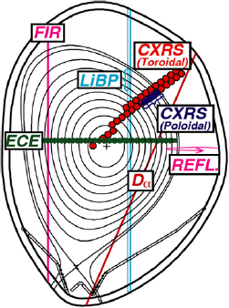
Figure 1. Plasma cross-sectional shape with diagnostics for discharge E049219.
Download figure:
Standard image High-resolution imageFigure 2 shows the time evolution of a balanced neutral beam injection (NBI) discharge E049219. It is clear that the Dα signal begins to decrease smoothly at a L–H transition ( = 0.0 s) when the edge Er becomes increasingly negative at about 200ms after the additional NBI heating, indicating the ETBs formation as seen in the enhancement in the pedestal temperatures for both ions and electrons as well as the plasma stored energy.

Figure 2. Waveforms for discharge E049219. (a) NBI power, plasma stored energy, ion and electron temperatures at the top of pedestal, (b) line averaged electron density and Dα emission, (c) radial electric field and density fluctuation measured by Reflectometry, and (d) frequency and time resolved spectrogram for the toroidal mode of n = 0 component in the magnetic fluctuation detected by the sum of eight channel saddle loop arrays (toroidal), including the predicted GAM frequency at the normalized radius of 0.9 (dashed line).
Download figure:
Standard image High-resolution imageThere are two time-scales in the changes in the Dα. One is characterized by a slow L-H transition with the time-scale of the decay in the Dα value of ~100 ms in the initial ELM-free H-phase (0.0 s ⩽  ⩽ 0.32 s), as a rise in both temperature and density in association with the change in the Er (down to −40 kV m−1) at the plasma edge region. The other is complex multi-stage Er-transitions with a fast time-scale of ~1 ms (or less) in the later ELM-free H-phases (0.32 s ⩽
  ⩽ 0.49 s), exhibiting a transient hysteresis in the forward and backward Er changes [22].
It should be noted that the slow initial H-phase can be seen not only discharge E049219, but also other discharges in JT-60U at lower IP/BT condition, such as 1.0 MA/2.6 T at similar q95 ~ 4. While the mechanism of L–H transition having different time-scale from conventional tokamaks is not well understood so far, we should remind that the usage of different heating schemes, such as NBI, ECH, ICRF, and so on, could affect the types of L–H transition, especially for the perpendicular NBI that was used on JT-60U for both heating and diagnostic (CXRS). On the other hand, the observation of the Er-transition having a fast time-scale (following a slow L–H transition) as seen in the conventional tokamaks during the L–H transition is not 'typical' of other discharges in JT-60U at lower IP/BT conditions. At a typical lower IP/BT conditions, we observed the ELM-free H-phase after a slow L–H transition at shorter intervals than that for discharge E049219 and following Type-I ELMing H-phases without the successive 'forward'/'backward' sharp transitions in the later phase as some sort of dithering H-mode phase that is very specific to the JT-60U tokamak under strong ion heating and high toroidal magnetic field conditions in association with the lower collisionality regime [23]. Instead, we could see only 'forward' sharp transition (following a slow L–H transition) just before the 1st large Type-I ELM at lower IP/BT conditions with lower density.
As seen in figure 2(c), the density fluctuation measured by Reflectometry at the pedestal region becomes smaller (or larger) in association with the changes in the Er. It should be noted that the density fluctuation data is the integrated value from the pedestal bottom to top, including the position at which the electron density gradient has its local Max. value. Its power spectrum exhibits a broad frequency dependence, which is sensitive to  ~ O(1) [24], and hence we use its frequency-averaged value (e.g. 10 ⩽ |f | ⩽ 300 kHz). It should be noted that the Reflectometry data is only available at the later H-phase. On the other hand, it is not available at the initial H-phase, since the pedestal electron density is lower than that for the its cut-off value (
 = 1.4 × 10¹⁹ m−3). At the later H-phase, it becomes clear due to increase in the pedestal density and its gradient.
Here, we point out the presence of the magnetic fluctuation having the toroidal mode number n = 0 (poloidal mode number m ~ 2) at or near the inferred frequency range of geodesic acoustic mode (GAM),  (the
(the  is sound speed, and
  is major radius [25]). The frequency of GAM is estimated at the top of pedestal during the initial H-phase just before the fast Er-transition (figure 2(d)). It should be noted that the GAM oscillation (n = 0) involves the m = 1 component for the density fluctuations, and hence it is accompanied by a weak magnetic one having m ~ 2 [26, 27]. As discussed in [28], one can speculate the turbulence driving forces that could cause the Er-bifurcation at the onset of GAM, since the GAM could be predominantly excited through a localized Reynolds stress force. This will be discussed further in the section 5.
Comparing the temperature profiles between ions and electrons in more details (figure 3), it is interesting that the pedestal structure for ion temperature represents a steeper gradient than that for electrons for both initial and later H-phases, as illustrated in figures 3(a) and (d). On the other hand, the pedestal density gradient both for ions (impurity) and electrons becomes larger as that seen in the ion temperature in association with the edge Er-well formation down to −40 kV m−1 at the initial H-phase as shown in figures 3(b), (e) and (f). The local Max. values of inverse gradient scale-length for the ion temperature ( ), impurity ion density (
 ), and electrons density (
 ) were found at which the Er has its Er-well bottom value (corresponding to the
  (curvature)-hill top value), while it is hard to see for the electrons temperature (
 ) due to a diagnostic limitation for the spatial resolution using a linear-fitting (instead of the tanh-like fitting). It is also interesting that the width in the
  (~6 cm) seems to be somewhat wider than that for the
  and/or
  (~5 cm), suggesting a difference in the particle transport between ions (impurity) and electrons. It should be noted that the change in Er-well bottom value from initial to later H-phases was about twice from −40 kV to −80 kV (corresponding change in Z value was four times or more) as shown in figures 3(b) and (c), while the pedestal gradients increased only by 10%–20% (or less).
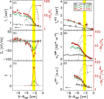
Figure 3. Radial profiles for discharge E049219. (a) Ion temperature and its inverse gradient scale-length, (b) radial electric field, (c) Z (non-uniformity of Er), (d) electron temperature, (e) electron density and its inverse gradient scale-length, and (f ) ion (fully stripped carbon impurity ion) density and its inverse gradient scale length. Vertical hatched lines correspond to the location at which the Er has its well bottom (i.e. Er-curvature hill top) value.
Download figure:
Standard image High-resolution imageAs shown in figures 4(a) and (b), we found that both ion and electron density gradients have been developed from  = 0.27 s to 0.33 s (1st forward Er-transition), while an improvement in the particle transport for electrons seems to be rather weaker than that for ions during an initial H-phase, suggesting a difference in the turbulence transport due to particle source. During the backward Er-transition from
  = 0.33 s to 0.40 s, both
  and
and  values decrease, while the
  becomes larger with essentially the same
  . Furthermore, we found the 2nd forward Er-transition from
  = 0.40 s to 0.47 s with essentially the same total confinement property, excepting a change in their pedestal width [19, 29].

Figure 4. Relationship of inverse gradient scale-length between ion (impurity) and electron channels for discharge E049219; (a) temperature, (b) density, and (c) pressure. The radial positions are at which the Er has its well-bottom value (corresponding normalized radius, r/a ~ 0.96).
Download figure:
Standard image High-resolution imageAs can be seen in figure 4(c), improvement in the total transport for electrons was confirmed, while it seems to be delayed as compared to (and be smaller than) that for ions (impurity) as seen the relationship for the inverse gradient scale-length between ions,  and electrons,
  . It is also suggested that both thermal and particle transports for each species of plasma (i.e. either ions or electrons) respond in their own time-scales in association with the change in the Er. This observation will be discussed in the next section.
3. Inhomogeneous Er-effects on ion and electron transport channels
A better understanding of how the edge Er regulates the system for each transport channel could lead to an improved accuracy for predicting and interpreting the complex behavior of plasma as self-organized system.
The focus of the study of the turbulence suppression was first made on the slow transition phase. As a result of a detailed comparison between an experiment and theoretical model, we have confirmed the non-uniformity of Er on the ETBs formation, quantitatively.
As shown in figure 5(a), we found a significant reduction in the ion thermal transport,  , during an initial H-phase having a weak Er value (corresponding Z value was less than unity) towards the neo-classical level, while no further reduction in the
  as the Z value became larger in the later H-phase.
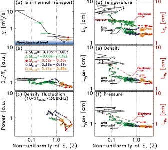
Figure 5. Dependence on the non-uniformity of Er (Z) at the pedestal (discharge E049219). (a) Ion thermal transport coefficient at the pedestal region, (b) Dα signal normalized by the edge line-averaged electron density, (c) density fluctuation, scale-lengths of (d) temperature, (e) density, and (f ) pressure for ions (impurity) and electrons.
Download figure:
Standard image High-resolution imageOn the other hand, reduction in the electron thermal transport (evaluated by the  value) was only 20% (or less) during an initial H-phase as shown in figure 5(d). Furthermore, we could not see any significant changes in the
  (as well as the
  ) in the later H-phase at 0.32 s ⩽
  ⩽ 0.36 s, while the
  value became shorter at 0.36 s ⩽
  ⩽ 0.41 s even at the later H-phase, keeping its value until
  ⩽ 0.49 s. This observation suggests that the non-uniformity of Er may not be directly connected with the electron thermal transport solely, while we should pay more attention to its effect on both thermal and particle transports, and their energy transfers. Furthermore, we found a difference in the dependence on Z of the
  and
and  during a slow L–H transition as shown in figures 5(d) and (e). The impurity density gradient becomes larger at Z ~ 0.1 (just after a slow L–H transition) as its well-known phenomena in the standard H-mode, while its change seems to be smaller than that for the ion temperature gradient. Indeed, the change in the
  value after a slow L–H transition seems to continue during a initial H-phase up to Z ~ 0.5, and the
  value begins to decrease. It should be noted that the temporal responses for the electron density and temperature gradients are also different. These experimental observations described above suggest the presence of multiple types of turbulent plasma state, which will be useful for the theoretical model validation and testing in simulation. This will be discussed in section 5 in more detail.
During the later H-phase, including both forward and backward Er-transitions, we found a clear and further response of the particle transport, which is interpreted from  and
and  in addition to the change in the Dα signal normalized by the edge line-averaged electron density,
  (as utilized for a better indicator for the particle transport) as shown in figures 5(b) and (e). It seems to be consistent with the abrupt changes in the edge density fluctuation (which is sensitive to the
  ~ O(1) [24]), following the change in the non-uniformity of Er at a stronger Z (⩾1) regime as illustrated in figures 5(b) and (c). It should be noted that the particle transport seems to be reduced even in an initial H-phase during the slow L–H transition as inferred from
  value at a smaller Z value of less than unity.
4. Nonlinear dynamics inducing the electric field bifurcation
Addressing the remaining issues relating to the mechanism of the Er-bifurcation, the nonlinear dynamics of multiple transition processes with different time scales are studied. We have identified the change in the radial current structure by using a Poisson's equation;
where  is the relative dielectric constant of toroidal plasmas [30–33].
As illustrated in figure 6, we found a broad and weak j r peak around the pedestal region at the slow L–H transition, while a highly localized and stronger j r was generated during Er-transition at the later H-phase. It should be noted that a required j r peak for the slow L–H transition (occurred at the normalized Er value of  < 1, where the
  is poloidal gyro-radius for ions) is estimated to be sufficient 1/10 order (or less) of that for the forward Er-transition during a later H-phase (occurred at
  ).
).
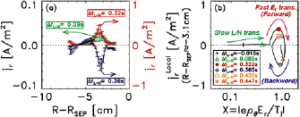
Figure 6. (a) Radial current structure (discharge E049219). Relationship between the local radial current and normalized Er-parameter at R-RSEP ~ −3.1 cm is also shown in (b).
Download figure:
Standard image High-resolution imageFurthermore, it is interesting that a local j r value for the backward Er-transition is comparable with that for the forward Er-transition as well as its time-scale, but being opposite in sign. So that, it is suggested that the plasma could keep a pedestal structure having a weak Er after the backward Er-transition. This finding suggests the contribution of different processes associated with the radial current: for example, the loss-cone loss, the neoclassical bulk viscosity, the Reynolds stress, the wave convection, and the charge exchange, etc, which could cause the onset of complex multi-stage Er-transitions described above.
5. Discussion on a multiple types of turbulent plasma state
Experimental observations described above suggest the presence of multiple types of turbulent plasma state (e.g. electron temperature gradient, ETG, or trapped electron modes, TEMs, and ion temperature gradient, ITG, turbulent regimes [34–36]). We discuss here the probability of accessing the multiple turbulent states due to the distinct Er-effects for various transport channels, depending on the non-uniformity of Er value.
The first of these types can be seen at Z = 0.1–0.3 regime, which is responsible to the anomalous transport of ion energy (e.g.  ~ 0.1).
The second one is at a higher Z (⩾1) regime, which is effective in reduced particle and/or electron transport, having higher wave numbers (e.g.  ⩾ 1). The suppression of anomalous transport of ion energy with lower wave number proceeds in the lower Z (<1) regime, and then remaining one with higher wave numbers continues to respond up to higher Z (⩾1) regime.
Furthermore, there might be another type at an intermediate Z regime, where the electron transport stays unchanged (or becomes larger) in comparison with the L-mode state. Indeed, we found that the turbulence amplitude (evaluated by the magnetic signal with n = 0 oscillation at the frequency of GAM predicted at the normalized radius of ~0.9) becomes larger with increasing the temperature gradient non-lineally at Z ~ 0.5 regime as shown in figure 7.
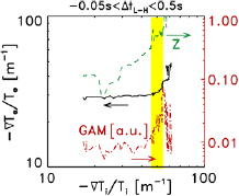
Figure 7. Dependence on inverse-gradient scale-length for the ion temperature to the inverse-gradient scale-length for the electron temperature (black solid line), non-uniformity Er-effect at the pedestal (green dashed line), and turbulence amplitude evaluated by the magnetic signal with n = 0 oscillation at the frequency of GAM predicted at the normalized radius of ~0.9 (red dash dotted line) for discharge E049219 during the time relative to the L–H transition from −0.05 s to 0.5 s.
Download figure:
Standard image High-resolution imageAs discussed in [36], trapping of turbulence clumps by the GAM is the key parameter for determining either suppress or enhance turbulence, while it is likely that ITG-driven turbulence is the main source for zonal flows and GAM fluctuations. Unfortunately, it seems to be very difficult for identifying the radial structure of the GAM in the H-mode plasmas due to diagnostic limitation, and hence we could not discuss whether ITG-driven short-wavelength eddies act like shear flows and suppress ETG turbulence in this study.
Also, it is still unknown whether the higher k mode appears after suppression of lower k mode (at which the slow L–H transition takes place), or coexists from the beginning (i.e. L-mode phase), although the phenomenology of this multichannel transport appears to be theoretically rich and complex, suggesting the presence of the cross-scale interaction [37].
6. Summary
Based on the criterion proposed in [15] [ ], we investigated the cause of the complex multistage transition in the JT-60U H-mode edge in terms of a possibility of the presence of multiple types of turbulent fluctuations in the ETBs region.
We found that the non-uniformity of Er affects the ion energy and other channels of transport differently; One is responsible to the anomalous transport of ion energy (e.g.  ~ 0.1–0.3), and the other is effective in enhancing particle transport, having higher wave numbers (e.g.
  ⩾ 1). The suppression of anomalous transport of ion energy with lower wave number proceeds in the lower Z (⩽1) regime, and then remaining one with higher wave numbers continues to respond up to higher Z (⩾1) regime. Furthermore, there might be another type having an intermediate wave numbers (e.g. 0.5 ⩽
  < 1). If so, we should consider not only the different scales such as ITG, TEM, and ETG, but also the presence of their cross-scale interaction [37], as well as the differences in the turbulent transport between main ions and impurities as a future problem.
These analyses presented here, showing multiple turbulence states and associated bifurcation dynamics, contribute to the understanding of the L–H transition condition. Indeed we could see multiple types of turbulent plasma state, being accessible by a distinct Er regime that are very specific to the JT-60U H-mode edge condition (e.g. slow L–H transition and following multi-stage Er-transitions during H-mode phase). If we had precise Er measurements in the core, this would help in improving our understanding of ITB formation [38], which should be useful for theoretical model validation and testing in simulations.
One of the most important remaining issues is experimental identification of the generation mechanism of the edge Er in terms of the generation of the edge radial current, while the phenomenology of this nonlinear dynamics of multiple transition processes nevertheless remains theoretically rich and complex. A more detailed comparison between the experimental data and theoretical model could help identifying the main mechanisms.
Acknowledgments
The authors deeply appreciate the continued research and operational efforts of the entire JT-60 team. Discussions with Drs P.H. Diamond, U. Stroth, J.Q. Dong, K. Ida, T. Kobayashi, and M. Yagi are also acknowledged. Authors acknowledge the partial support by Grant-in-Aid for Scientific Research (JP 15K06657, JP 15H02155, JP 16H02442) and collaboration programs between QST and universities and of the RIAM of Kyushu Univ., and by Asada Science Foundation.
Appendix
An example of the quality of data available from JT-60U tokamak measured by CXRS with high precision is shown in figure A1. The location at which the inverse gradient scale-length for the ion temperature,  , is defined by the radius from the separatrix, R-Rsep = r0, at which the Er-profile has its well bottom value (corresponding the local Max. Er-curvature hill top as the Z2 term).

Figure A1. Radial profiles in the stationary H-mode plasma (discharge E049228): (a) ion temperature (Ti), its radial derivative ( ) and inverse gradient scale-length (
 ), (b) radial electric field and its shearing rate (
 ), and (c) Z (non-uniformity of Er). Vertical solid (r0) and dashed (r1) lines denote the locations at which the
  and
and  have their own local peak values in the pedestal region, while the dashed (r+) and dash dotted (r−) lines exhibit the location at which the
  has its local Max. and Min. values.
Download figure:
Standard image High-resolution imageLooking at figure A1(b), one can see that the location of r0 is at which the local effect of the  (corresponding the local Er-shear) vanishes, while the location at which the
  has the local Min. values (defined as r-) exists more inside from the location of r0 (e.g.
  1 cm).
Here, the E × B shearing rate for a shaped plasma [39] are given by  . As it is frequently discussed, the shear flow stabilization effect for the turbulence suppression is expected regardless of its sign according to the theoretical prediction, while the region at which the radial electric field has the local Max.
  value (defined as r+) exists more outside from the location of r0 (e.g.
  1 cm). Therefore, there is no local beneficial effect of the Er-shear effect (i.e. Z1 term), or rather the experimental data can support the favourable effect of the positive Er-curvature hill (i.e. Z2 term) as predicted by the theory on the ETB formation due to turbulence suppression, where the scale-length of the ion temperature gradient,
  , becomes close to that of the ion poloidal gyro-radius,
  .
.
On the other hand, the location at which the ion temperature profile has the local Max.  value (defined as r1) always exists slightly inside from the location of r0 (e.g.
  1 cm), exhibiting that the location of r1 is in between r− and r0 (i.e.
  ). In terms of the experimental point of view (such as diagnostic limitation), it seems to be hard to separate which is more essential location for an indicator of the transport improvement, r0 or r1. If one can use the location of r1 instead of r0, it results in leaving the location of r+ far-away from the transport improvement region (i.e.
  ). Therefore, it is considered that the location of r0 (i.e. local Max. inverse gradient scale-length value) seems to be better for the comparison between a transport improvement and inhomogeneous Er-effects (i.e. Z2 and/or Z), as adopted in this study, instead of r1 (i.e. local Min. radial derivative value). It should be worth noting that both
  and
and  profiles become close to zero value (within their error bars) at the separatrix (i.e. R-Rsep ~ 0) as well as Er-shear and curvature profiles.
The most important point of this discussion is how much accuracy for the positional relationship between the pedestal parameters and Er. As discussed in the previous publications, one of the advantages for CXRS measurements is that the diagnostic could measure the pedestal parameters for the carbon impurity ions, simultaneously, which makes it possible to evaluate their radial derivatives and Er at the same radial coordinates.
It should be noted that the CXRS data used in figure A1 are averaged one at the onset of ELM, being extracted from all sampling data during the inter-ELM phases from 6.0 to 7.3 s (discharge E049228). As shown in figure A2, there is variation in the position of the separatrix of about ± 1 cm (or more) due to change in the global equilibrium parameters (such as internal inductance and/or beta) during the ELM cycles under a plasma positional control. Using its variation as a natural radial sweeping of the plasma in terms of the diagnostic points, we could achieve a higher spatio-temporal resolution [40], overlaying the data onto the radius along to the magnetic axis (see, figure A3).
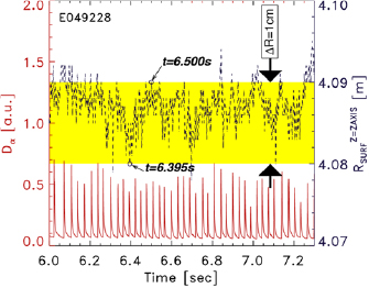
Figure A2. Waveform for the Da emission and the major radius of separatrix at the vertical position of the magnetic axis (discharge E049228).
Download figure:
Standard image High-resolution image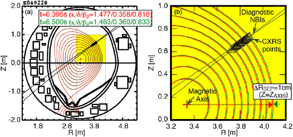
Figure A3. (a) Two typical magneto-hydrodynamic equilibria (t = 6.395 s in red and t = 6.500 s in green) for discharge E049228. Geometrical layout of the perpendicular neutral beam injection lines together with the CXRS diagnostic is also shown. (b) Expanded view of (a).
Download figure:
Standard image High-resolution image
Furthermore, there is another systematic uncertainty for radial positions of the diagnostic points due to an error during data mapping process, since there should be unavoidable errors for an absolute calibration for each diagnostic. One is absolute positional calibration for both magnetics and CXRS, including a relative uncertainty in term of the vacuum vessel. The other is the sensitivities for magnetic sensors, being used for the magnetic equilibrium reconstruction. As illustrated in figure A3(a), one can see that both magnetic equilibria between t = 6.395 s and 6.500 s seem to be almost matched. However, we found systematic differences between them by a more detailed comparison as shown in figure A3(b). As a result, even if there is variation of only ~1% in the equilibrium parameters (such as κ/δ/βp), systematically, it is suggested that data mapping process could result in the systematic shift (e.g. an avoidable error) of the separatrix position of an order of 1 cm, regardless of inward or outward direction.
It is well known that the pedestal gradient structures just inside the separatrix (such as edge toroidal current and/or magnetic shear) also cause another systematic uncertainty, since internal current profiles can affect the separatrix shape, in particular around the X-point. However, it is also difficult for taking that into account for the magnetic equilibrium calculations utilized here, since it is difficult to measure except for a few demonstrations of the proof of principle. This issue should be left for future study.