


Abstract
We present state-of-the-art computations of propagation and absorption of electron cyclotron waves, retaining the effects of scattering due to electron density fluctuations. In ITER, injected microwaves are foreseen to suppress neoclassical tearing modes (NTMs) by driving current at the  and
and  resonant surfaces. Scattering of the beam can spoil the good localization of the absorption and thus impair NTM control capabilities. A novel tool, the WKBeam code, has been employed here in order to investigate this issue. The code is a Monte Carlo solver for the wave kinetic equation and retains diffraction, full axisymmetric tokamak geometry, determination of the absorption profile and an integral form of the scattering operator which describes the effects of turbulent density fluctuations within the limits of the Born scattering approximation. The approach has been benchmarked against the paraxial WKB code TORBEAM and the full-wave code IPF-FDMC. In particular, the Born approximation is found to be valid for ITER parameters. In this paper, we show that the radiative transport of EC beams due to wave scattering in ITER is diffusive unlike in present experiments, thus causing up to a factor of 2–4 broadening in the absorption profile. However, the broadening depends strongly on the turbulence model assumed for the density fluctuations, which still has large uncertainties.
Export citation and abstract BibTeX RIS
1. Introduction
In order to obtain stable operation of a tokamak reactor, instabilities endangering the confinement or performance of the plasma need to be controlled, preferably in automatic manner. One of such instabilities is the neoclassical tearing mode (NTM) [1]. In existing machines, NTM mitigation and suppression has been successfully obtained using electron-cyclotron current drive (ECCD) to replace the missing bootstrap current inside the magnetic island [2]. The effect relies on the ability to focus and steer electron-cyclotron (EC) beams by mirrors, thus enabling accurate localization of the driven current profile. This demands accurate knowledge of the equilibrium, i.e. the location of the resonance surface where the beam will be aimed at. By controlling injection angles (poloidal/toroidal), the necessary amount of current can be driven inside the NTM island to stabilize it. Correspondingly, effort has been applied to predict whether such a control system is plausible for ITER [3, 4]. Based on these analyses, the EC upper launcher (UL) has been assigned mainly to control NTMs [5–8]. During the development of the UL EC system, several physics phenomena possibly jeopardizing the stabilization of NTMs have been identified [9]. Out of these phenomena, the most important and still difficult to quantify issue is the beam broadening by scattering due to turbulent density fluctuations and this paper aims to give more insight in this area using state-of-the-art modeling.
When the injected microwave beam propagates in the plasma, density fluctuations act as random lenses and refract the beam. The effect of these fluctuations on beam broadening depends on the fluctuation characteristics and the relative position of the fluctuations to the resonance surface where the current is to be driven. Since these factors are particularly favorable for existing machines, most importantly the beams have a short propagation distance between the fluctuation regime and the absorption regime, beam broadening is expected to be small and hence fairly difficult to measure. However, some evidence of such of an effect has been recently reported [10] and more is put to further investigate the issue experimentally. Simultaneously, modeling efforts have been reported to study this effect [11–15].
Unfortunately, most of the modeling tools, like beam or ray tracing codes, are not applicable in the presence of small scale fluctuations. The current work aims to address these issues with simulations performed using the wave kinetic approach. The turbulent fluctuations can be assumed to be frozen in the plasma—characteristic velocities of turbulent structures are much smaller than the beam group velocity and at the same time the beam power is on over several turbulence turnover times. Therefore, the effect of turbulence can be studied by averaging over a large number of realizations of the turbulent field or by means of the formalism of the wave kinetic equation which allows us to derive an averaged scattering operator describing directly the average effect of turbulence on the beam. While the former strategy is usually adopted by full-wave codes [16], the latter is the choice of WKBeam code [17] used in this work. The main advantage of this reduced model is the reduced cost of the computations, while keeping the key physics in the model, namely, beam diffraction, scattering (adopting the Born approximation as described below), absorption and full axisymmetric tokamak geometry. The scattering operator in general includes the possible scattering from the launched mode to secondary mode [18] that has been studied also by analytical methods [19]. In the case of ITER, power converted from first-harmonic ordinary to extraordinary mode is reflected at the corresponding cut-off at the plasma boundary, thus causing stray radiation [48]. However, cross-polarization scattering does not lead per se to beam broadening and will not be discussed in this paper.
After this introduction, in section 2, we present the theory behind the WKBeam code and give a short overview of the scattering operator. Verification and benchmarking studies are briefly discussed to build trust on the implementation of the theory. We will present the model to be used for density fluctuations. The underlying radiation transport process is discussed in detail. For focused beams, the impact of turbulent fluctuations on beam broadening increases with machine size. The effect is predicted to be large for ITER, but a measurement of the effect is difficult on existing machines. Moreover, depending on the parameters, the radiative transport can be diffusive or superdiffusive. In present-day experiments like ASDEX Upgrade, the transport tends to be superdiffusive, which leads to the formation of elevated tails in the absorption profile but a limited reduction of the peak absorption. On the other hand, the same analysis indicates that ITER lies in the diffusive regime. In section 3, we will introduce the main inputs of the studied 15 MA ITER H-mode scenario, together with the beam and mirror parameters. We will show the absorption profiles of the beams with and without the fluctuations and also present relevant scans over the input quantities that cannot be realistically extrapolated to ITER. Results show up to a factor of 2.5–4.5 broadening in the deposition profiles compared to the case without fluctuations. In section 4, we discuss the implications of our results to NTM control in ITER.
2. Theoretical background and numerical models
2.1. Wave kinetic equation
The wave kinetic equation with random fluctuations was originally formulated in [20] adapting a statistical approach proposed by Karal and Keller [21] in combination with Weyl-symbol calculus for the phase-space representation of the wave field [22]. The specific form of the wave kinetic equation relevant to coherent wave beams and implemented in WKBeam [17] is usually written in coordinates normalized to the scale L of the equilibrium plasma profiles so that the semiclassical parameter  appears explicitly in the theory; here ω is the launched frequency, c the speed of light in free space, and
  is the wave number in free space. It is important to note that the scale length L refers to the background plasma equilibrium which does not include turbulent fluctuations. Hence the parameter κ is large even in presence of short-scale fluctuations and the semiclassical limit
  can be considered, yet not directly on the solution of Maxwell's equations for the wave field, but rather on the averaged wave energy density, which is represented by the averaged Wigner function. The wave kinetic equation describes the statistically averaged Wigner function of the beam in the limit
  . We refer to Weber [17] for a sketch of the derivation. Here instead we start from the wave kinetic equation written in physical coordinates as appropriate for the application. It reads

where, for each cold plasma propagation mode (namely the ordinary mode (O-mode,  ) or the extra-ordinary mode (X-mode,
  )) labeled by Greek indices,
  is the Hamiltonian of standard ray-tracing theory [23, 24],
  the absorption coefficient,
  the scattering operator to be discussed below in more detail. The unknown is the statistically averaged Wigner function
  which depends on the spatial coordinates x and the refractive index N. The left-hand side is written in terms of canonical Poisson brackets on the
  phase space, given by

One should notice that the wave kinetic equation has the form of a steady-state kinetic equation with an additional constraint. The Wigner function can be associated to the electric field energy density. It has an analogous role to distribution function of the kinetic theory as we can derive integral expressions over the Wigner function for any quantity that can be written in terms of  , where E is the electrid field. An example of such a quantity is, e.g. the absorption profile. The constraint merely means that there is no energy on phase-space points that do not satisfy the dispersion relation of the mode,
  . Further details on the Monte Carlo solution of the wave kinetic equation and on how to construct such integrals of Wigner function are given in [17].
In the WKBeam code, the Hamiltonians  are computed from the Hermitian part of the dispersion tensor
  with
with  being the Hermitian part of the dielectric tensor [25] and
  the polarization unit vector of the mode α.
The absorption coefficient  , on the other hand, is computed from the hot-plasma dielectric tensor accounting for relativistic electron-cyclotron resonance interaction. More specifically, one can write
  where
where  is the imaginary part of the refractive index vector which is computed in the WKBeam code by the same routines used in the complex-geometrical-optics code GRAY [26] and the paraxial WKB code TORBEAM [27].
The general form of the scattering operator includes cross-polarization scattering terms from mode α to mode β and is given by
where the integration is over the refractive index space. Here the scattering cross-section
describes a momentum-preserving three-wave interaction process in which a mode α carrying refractive index N interacts with turbulence exchanging momentum  and thus scattering into a mode β with refractive index
  , with momentum conservation
  . The spatial position is not changed in the scattering event. The variation in momentum
  is provided by the turbulence spectrum Γ which is rigorously defined as the Wigner transform of the two-point correlation function of the relative electron density fluctuations
  , namely,
where ne is the average electron density profile of the plasma and s is an integration parameter. Here the term inside  corresponds to the two-point correlation function of the electron density fluctuations.
In the WKBeam code, the two-point correlation function of the electron density fluctuations is a critical input quantity. Such information is usually not easily recovered, neither from experimental data nor from simulations. Therefore we make use of a model which is based on the current theoretical understanding of turbulence in a magnetized plasma, thus reducing the required inputs to quantities that can be inferred from available data. The model used in this work amounts to

where  is a scalar function accounting for the spatial localization of turbulent density fluctuations and

is a tensor accounting for the anisotropy of turbulence in magnetized plasmas,  and
and  being the correlation lengths in perpendicular and parallel directions with respect to the unit vector b of the equilibrium magnetic field. The Gaussian shape arising from broad-band (white noise) signals is a good approximation for a range of plasma conditions as supported by experimental measurements, e.g. [28–30]. The input parameters for the code are thus reduced to the function F, which is usually specified on the poloidal plane of the tokamak and the two correlation lengths, see section 2.3 below. The function F in particular can be identified with the root-mean-square density fluctuations: In fact, we have, upon setting
  ,
,
and the average here is a statistical average (no spatial averaging should be performed). A further advantage of this model given by equation (7) is that the integral in spectrum Γ can be computed analytically.
2.2. An estimate of the effect of density fluctuations
The effect of the scattering operator on the solution of the wave kinetic equation can be rather complicated and it is in general not just a diffusion process. We can in fact distinguish two radically different regimes (as shown in section 2.5), namely, a superdiffusive regime in which scattering deforms the tails of the wave energy distribution only with little consequences for the quality of the beam, and a diffusive regime in which the whole wave energy distribution spreads with a significant broadening of the beam. An indication of the scattering regime can be obtained from the total scattering cross-section
which is the average number of scattering events per unit of propagation length for the mode α and near the phase-space point  . If
. If  is the distance traveled by a beam in the turbulent plasma, then

where  is the average of
  along the beam path (reference ray), gives an estimate of the average number of scattering events for that beam. For
  we expect to have diffusive solutions with significant broadening of the beam. It is therefore useful to have simple estimates for such a parameter.
We begin with the analytical calculation of the spectrum Γ, which in view of equation (7) amounts to
where we have introduced the parameters  and
and  that play the role of spectral widths and cylindrical coordinates defined by

with  being an orthogonal reference frame constructed around the unit vector b of the local magnetic field.
Turbulence in a magnetized plasma is well within the limit  both because of the high frequency of the wave and the elongated structures of the turbulence along the magnetic field direction (
 ). Hence we can consider the limit
  , for which one has
The presence of the Dirac's delta-function together with two key properties of the cold-plasma dispersion tensor allow us to compute the total cross-section exactly. The key properties are: (i) The dispersion relation  corresponds to
  with
with  a known function; (ii) The dispersion tensor and thus the polarization vectors
  depend only on
  and not on the polar angle
  . Particularly (i) implies
In view of such properties and in the limit  , we obtain
where  has been evaluated 'on-shell', i.e. on the dispersion surface
  , and we have defined the matrix of coefficients
where both  and
and  should be evaluated at
  , while the term in square brackets should be evaluated at
  and
and  .
.
The remaining integral can be computed by means of the Jacobi–Anger expansion,
where  are the Bessel functions and the sum is over the set
  of integer numbers. We can use this identity with
  and
and  and only the term
  gives a contribution. At last we obtain
and  are the modified Bessel functions of first kind and, in particular, I0 is even so that
  .
.
Expression (10) is strictly only valid under the assumption of long parallel correlation length  which is usually satisfied in cases of interest. If in addition, we consider the limit
  , which is often the case for beams in the EC frequency range, the Hankel's large-argument expansion of the modified Bessel function,
yields the simpler expression
which exhibits the linear dependence with  .
.
With the aim of practical estimate of scattering, however, it is convenient to further simplify the expression for  . In most cases the toroidal injection angles are modest (<20 degrees), hence we consider the simple case of perpendicular propagation. In the reference frame in which the local magnetic field defines the third axis and the refractive index belongs to the plane spanned by the first and third axis (Stix reference frame [31]), perpendicular propagation implies
  . For the ordinary mode
  we find
where  is the electron plasma frequency. As a result, for perpendicular propagation,
Even under such simple conditions, the calculations for the extra-ordinary mode  , although doable, yield rather cumbersome results. In fact one has
with the proportionality constant for eX being determined by  and
and
where
are the standard parameters of the cold-plasma dielectric tensor and  is the electron cyclotron frequency (defined with the elementary charge so that it is a positive number). The dispersion relation
  in this case corresponds to
as expected, but the Hamiltonian HX has been computed as the eigenvalue of the dispersion tensor. Then we have
In this specific case of perpendicular propagation, the cross-polarization terms  and
and  are both exactly zero, no matter how close the mode dispersion surfaces are. This is due to the block-diagonal structure of the matrix
  with the polarization eO and eX being in the subspace of the two different diagonal blocks of the matrix. The fact that modes are exactly decoupled for perpendicular propagation independently of the fluctuation level can also be inferred directly by inspection of Maxwell's equations.
The expression for  is still rather complicated for practical use. Instead of an exact calculation one could consider an easier lower bound. This can be computed on noting that the maximum and minimum values of any quadratic form
  , where z is a complex vector satisfying
  and A a complex positive semi-definite Hermitian matrix, amount to the maximum and minimum eigenvalues, respectively. We can therefore obtain a bound for
  as well as for
  . Since we are interested in the X-mode for perpendicular propagation, we can limit our calculation to the blocks of the matrices orthogonal to the O-mode polarization and computing the eigenvalues we obtain

The lower bound on the derivative of HX cannot be used as we need  . That however allows us to obtain a lower bound for
  . In summary we have
for the ordinary mode while, with the lower bound for  ,
,
for the extra-ordinary mode, both results being valid for perpendicular propagation under the limits  .
.
A simple estimate of the parameter  can now be readily written by using either equation (13) or (14) as relevant to the considered mode. In order to compute
  rigorously we should average
  over the propagation path of the beam in the turbulent plasma. For simplicity however we can evaluate
  , which for perpendicular propagation depends on x only, at a given point in space chosen to represent the typical value of plasma parameter in the turbulent region. Then we can write an estimate for
  which can be evaluated for a given tokamak scenario without need of ray- or beam-tracing calculations. That is,
and we have introduced the cut-off density  . The authors would like to remind that this chain of approximations and simplifications were made to obtain a simplified expression for the categorization of the transport regimes. In the implementation of the code, the general expression (4) is evaluated during a scattering event as described in [32].
2.3. Model for density fluctuations
The turbulence model employed in WKBeam simulations consists in a model profile for the function F defined in equation (7), which is the root-mean-square relative electron-density fluctuations. We model F as a function of the radial coordinate  , where
  is the normalized poloidal flux (
 and
and  corresponds to magnetic axis and the separatrix, respectively), and the geometrical poloidal angle θ. At first we shall assume that F is a purely radial profile, i.e.
with Fr depending only on the radial coordinate  . The specific profile used for Fr was selected based on the experimental work in [33, 34] and it is shown in figure 1(a). It is a piecewise defined function combining core region until
  , a (linear) ramp-up region at
  and a constant edge region at
  . The core value in H-modes is a few percent (and has a negligible effect on the beam broadening), here it is chosen to be 2%. While the edge level dominates the beam broadening and here it was selected to be 20%. A Gaussian centred at
  is shown for comparison, as it has been used in the earlier works [11, 12]. Note that even though the function has rather high values outside separatrix, the fluctuation density itself is rather small due to small electron density. This is further illustrated in figure 1(b). As this extrapolation from current experiments to ITER is definitely uncertain, a scan for the edge value is presented in section 3.3. The correlation length was assumed to scale like
  –
– [35], where
  is the sound gyroradius. The authors are aware that this scaling might break down when going from open to closed field lines. As the temperature of the plasma is a radial function, so is the expected correlation length. In this paper, however, a constant value of the correlation length was used as the main effect of the fluctuations can be isolated to a radial domain close to the edge (we note, however, that the theory allows a radial dependency on the correlation length). Using ITER parameters, the correlation length in the studied scenario at the location of interest is 1-2 cm. Consequently, a value of 2 cm was used and a scan around this value is presented in section 3.3.
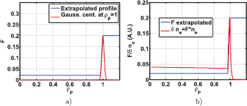
Figure 1. (a) Radial function F of the density fluctuation amplitude. Extrapolation from experimental H-mode profiles and a Gaussian profile centered at the separatrix are illustrated. In (b) we multiple the fluctuation amplitude profile by the background density, thus showing  (note, not in scale) as a function of the radial coordinate.
Download figure:
Standard image High-resolution imageIn the plasma core, the turbulence exhibits strong ballooning structure leading to poloidal dependency in the density fluctuation amplitude. According to recent 2D measurements combined with gyrokinetic modeling [36] suggest this ballooning behavior can be modeled (apart from fine-structure assumed to be not particularly important for the current application) using
where θ is the geometrical poloidal angle. For ITER, this ballooning leads to the shape illustrated in figure 2. In this figure the radial function shown in figure 1 was used. At the location where the UL EC beam enters the plasma, the value of the fluctuation amplitude is roughly half of the midplane value. However, only very marginal amount of information exists about the ballooning in open field lines either experimentally or theoretically [37–39], and even these observations are often of limited interest for us (limiter plasmas, L-mode). To compensate for these uncertainties, a scan over different fluctuation amplitude levels is performed, as detailed in the following sections.

Figure 2. Ballooning of the density fluctuation using equation (16). The amplitude of the fluctuations is normalized to peak value. Note that at the region where the microwave beam enters the plasma, the fluctuation amplitude is roughly half that of the midplane value.
Download figure:
Standard image High-resolution image2.4. Verification and validation studies
To ensure that the implementation of the theory is handled properly, several benchmarks have been carried out. These included a benchmark study without the fluctuations against well benchmarked and validated TORBEAM code [27]. Several different scenarios were studied, including various ASDEX Upgrade discharges and ITER. These cases involve variation in kinetic profiles, magnetic fields and also injection angles. Both the beam shape and absorption profiles were compared. In most of the cases, for which an ASDEX Upgrade example is shown in figure 3 and ITER examples in figures 4 and 5, both the beam and the profiles are extremely close to each other. However, some discrepancy in the absorption profiles were observed in particular for large toroidal injection angles like shown in figure 5. The reason for these discrepancies is thought to be a combination of physical differences between the codes (TORBEAM adopts the paraxial approximation, so that all the relevant information is computed on the central ray only) and the projection to flux surfaces necessary on the TORBEAM side when constructing the absorption profile.
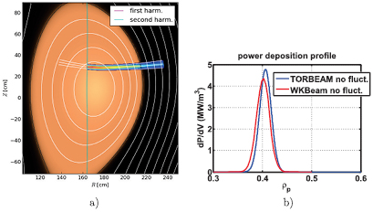
Figure 3. Comparison of the TORBEAM EC beam and WKBeam beam (a) and deposition profile as a function of  (b) in ASDEX Upgrade discharge #25 485. The beams are on top of each other, deposition profiles are not identical. Perpendicular injection with zero toroidal angle.
Download figure:
Standard image High-resolution image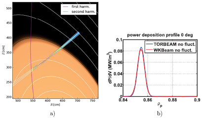
Figure 4. Comparison of the TORBEAM EC beam and WKBeam beam (a) and deposition profile as a function of  (b) in ITER. The beams are on top of each other, deposition profiles are on top of each other. This was carried out for a perpendicular beam injection.
Download figure:
Standard image High-resolution image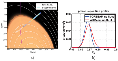
Figure 5. Comparison of the TORBEAM EC beam and WKBeam beam (a) and deposition profile as a function of  (b) in ITER. The beams are on top of each other, deposition profiles are similar. This was carried out for nominal toroidal injection angle of 20 degrees.
Download figure:
Standard image High-resolution imageFurthermore, the code was benchmarked against full-wave code IPF-FDMC [40]. In these studies, the effect of fluctuations on the beam shape was studied under ITER-relevant conditions, i.e.  . The main goal of this benchmark was to find the threshold above which the Born approximation, as introduced in the seminal paper by Karal and Keller [21] and applied to the wave-kinetic equation by McDonald [20], breaks down. See [17] for details in the implementation in WKBeam. This threshold is expected to be a function of the fluctuation amplitude and, therefore, a scan against this variable was carried out until the codes disagreed. The main result is that the WKBeam method agrees well with the full-wave calculations in the levels of fluctuations amplitudes expected in ITER, i.e.
  % as shown in figure 6. The beam broadening is here defined as the ratio of the fitted Gaussian widths of the beams with and without scattering. The WKBeam solution fits nicely on a second order polynomial fit represented by a solid curve in this figure. Therefore the basic physics assumption upon which the WKBeam code relies appears valid under ITER-like conditions.
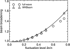
Figure 6. Demonstration of breaking down of the Born approximation using ITER relevant parameters. Full-wave and WKBeam codes agree well for fluctuation amplitudes  %. Solid curve represents second order polynomial fit to WKBeam data.
Download figure:
Standard image High-resolution image2.5. Transport regimes—comparison of AUG and ITER
As an example of present-day experiment, we take ASDEX Upgrade discharge #25 485. There the EC beam was in X-mode polarization with a frequency of 140 GHz. Using the information of the plasma quantities, we may construct a 2D map of the scattering parameter in equation (15) as a function of  and
and  as motivated by this equation. For this analysis, we have set a Gaussian layer around the separatrix, as illustrated in figure 1 and calculated the distance s the beam travels in this layer. The nominal values for the correlation length was 0.4 cm for AUG and 2 cm for ITER and the nominal amplitude was
  . In figure 7 we show the
  curve together with the nominal values of λ for the parameters discussed above. Clearly ITER is well in the diffusive regime, while AUG nominal values are close to boundary but on the super-diffusive side.
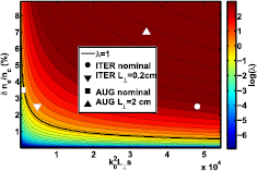
Figure 7. Transport regimes in AUG and ITER. Everything below  , like AUG nominal parameters, is superdiffusive and above, like ITER and AUG modified parameters, is diffusive.
Download figure:
Standard image High-resolution imageFor illustrative purposes, we considered also modified cases with  cm and
  for AUG and
  cm for ITER. With these parameters, the scattering parameter ends up clearly on the diffusive side in the AUG case and close to the boundary in ITER case. As the derivation of the scattering parameter includes several approximations, the boundary cannot be considered to be sharp. Moreover, the real transport, within the limits of our model, can be obtained by running the code and it was done for the two cases discussed above. The resulting statistically averaged electric energy density
  after the fluctuation layer as a function of a distance along the perpendicular distance to the EC beam is illustrated in figures 8 and 9. The diffusive beam shape in both cases can accurately be fitted with a Gaussian while the superdiffusive case has characteristic high tails, that suggest a Kappa or Lévy distribution [41, 42]. The ASDEX case is shown in figure 8. Red curve is a solution with out fluctuations, blue curve the solution using nominal parameters that produce superdiffusive behavior and green curve a modified turbulence case that produce a diffusive solution. For the latter two, points represent a fit (as described below). The ITER case is shown in figure 9. Here blue line is the case with out fluctuations, red line is the nominal diffusive case and green one is the superdiffusive example obtained using modified turbulence parameters. Again, the dots corresponds to fits.

Figure 8. Shape of the EC beam after the fluctuation layer in AUG discharge #25 485 with diffusive (green line,  %,
%,  cm) and superdiffusive (blue line,
  ,
,  cm) parameters. Gaussian fit is suitable only for diffusive regime, while superdiffusive beam has characteristic high tails.
Download figure:
Standard image High-resolution image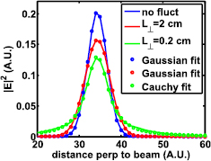
Figure 9. Shape of the EC beam after the fluctuation layer in ITER with diffusive (red line,  ,
,  cm) and superdiffusive (green line,
  ,
,  cm) parameters. Gaussian fit is very accurately modeling the diffusive and quiescent beam shape, while Cauchy fit is necessary for super-diffusive parameters with elevated tails.
Download figure:
Standard image High-resolution imageTo further illustrate the transport regimes, we fitted for the superdiffusive cases a generalized Cauchy distribution with
where  and c are free parameters of the fit. Using the beam shape coming from WKBeam to generate the least-square fit, c has a value of
  (95% confidence level), which is very close to Cauchy distribution (
 ). We have also counted the number of scattering events along each ray. In the diffusive regime, almost all rays (
 99%) have scattered at least once and most of them several times, whilst in the superdiffusive regime only a fraction of the rays undergo a scattering event (depends on how deep in the superdiffusive regime one lies, but here for example roughly 20%) and having more than one event for a ray is very unlikely. Last remark is the difference between the superdiffusive beam shapes of ITER and AUG examples, in ITER the high tails are more visible than in the AUG case. This can be explained by the fact that in AUG case the fluctuation layer is so short, and the scattering probability correspondingly low, that not enough scattering events occur to raise the tails, and the original Gaussian beam shape is retained rather well.
3. Results for ITER electron cyclotron upper launcher
3.1. Simulated scenarios
We have concentrated in this paper on the 15 MA  standard H-mode ITER scenario. It is the most important mission of ITER and thus it deserves special attention. Here we have modelled the flat-top phase according to the simulations presented in [43]4. The relevant 1D profiles of electron density and temperature are shown in figure 10 and flux surfaces of the equilibrium in figure 11 (the distorted shape around the X-point is due to an equilibrium re-processing and does not affect the results in the top region, where the beam propagates).
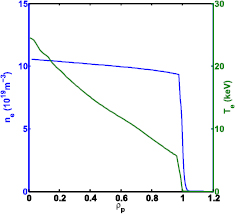
Figure 10. The kinetic profiles of electron density (left) and temperature (right) in 15 MA ITER scenario.
Download figure:
Standard image High-resolution image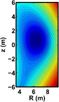
Figure 11. Flux surfaces of 15 MA standard H-mode scenario of ITER.
Download figure:
Standard image High-resolution imageRelevant parameters for the EC beams are given in table 1. Four different configurations are listed, namely the upper steering mirror (USM) and lower steering mirror (LSM) and both are separately optimized for current drive at  and
and  surfaces, where the most dangerous NTMs are expected to occur in the given scenario.
Table 1. Most important beam parameters for USM and LSM including both (2, 1) and (3, 2) resonance surfaces.
| Quantity | USM ( ) ) |
LSM ( ) ) |
USM ( ) ) |
LSM ( ) ) |
|---|---|---|---|---|
| Frequency (GHz) | 170 | 170 | 170 | 170 |
| Mode | O | O | O | O |
| Input power (MW) | 1 | 1 | 1 | 1 |
| Beam width (cm) | 5.047 | 4.813 | 5.047 | 4.813 |
| Focal length (cm) | 318.6 | 200.1 | 318.6 | 200.1 |
| Antenna R (cm) | 699.9 | 705.4 | 699.9 | 705.4 |
| Antenna z (cm) | 441.4 | 417.8 | 441.4 | 417.8 |
| Toroidal angle (deg) | 20 | 20 | 20 | 20 |
| Poloidal angle (deg) | 46.8 | 40.5 | 54.7 | 50.1 |
Resonance surface ( ) ) |
0.87 | 0.87 | 0.77 | 0.77 |
3.2. Absorption profiles and effect of ballooning
In figure 12 we show the absorption profiles of electron cyclotron beams. The set of profiles on the left-hand side of the figure (around  ) corresponds to deposition on the
  surface while the set on the right-hand side (around
  ) corresponds to the
  surface. Blue/black/red colour represents the case with 0/10/20% density fluctuation amplitudes, respectively, while the solid line shows the USM configuration and the dashed line the LSM configuration. An immediate observation is that the beams are broadened by a factor of ≈3 in all cases. Another peculiar feature of the scattered profiles is the non-Gaussian shape. This can be explained by a combination of beam-broadening-induced geometrical factors and aberration effects (these are naturally included in the model as each ray carries information of the refractive index N and also of the temperature that affects the absorption). The effect of density fluctuations is similar for both mirrors and both resonance surfaces, while the geometric distortion of the Gaussian shape is slightly stronger for the inner
  surface compared to the outer
  . Each of these simulations was performed using 4
 –2
–2 rays, which allows a statistically well-converged determination of the power deposition profiles.

Figure 12. Absorption profiles for both mirrors and both resonance surfaces with and with out the scattering of density fluctuations.
Download figure:
Standard image High-resolution imageOne major uncertainty of the density fluctuations on open field lines is related to ballooning. In the core region with nested flux surfaces, the fluctuations are strongly damped at the high-field side but only very scarce information is available for the open field line region of H-mode plasmas that is interesting for the present study. To evaluate the effect of ballooning on the profile broadening, we have assumed a core-like ballooning given by equation (16). A simulation was carried out for the USM  configuration, assuming 20% fluctuation amplitude at the outer midplane. For comparison, the results are shown together with 20% and 10% fluctuation amplitudes without ballooning in figure 13. As expected, the ballooning case is very close to the 10% fluctuation amplitude case as the level of fluctuations at the location where the EC beam enters the plasma is roughly half of the midplane value, in this case 10%.
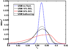
Figure 13. Absorption profiles with and without the ballooning in the density fluctuations.
Download figure:
Standard image High-resolution image3.3. Fluctuation parameter scans
Since some of the key input parameters have large uncertainties, a scan has been performed to assess the sensitivity of the results on these parameters. As a basis for this scan, we have selected the USM configuration for the  resonance surface. The scanned variables are the fluctuation amplitude
  and the correlation length
  shown in figure 14. In this figure we show the full width at half-maximum (FWHM) of the deposition profile compared to the quiescent case. It is readily noticed that the effect of fluctuations is to broaden the beam by a factor of 1.7 to 5.1, in the range of most likely fluctuation amplitudes by a factor of 2.5 to 3.5. In this scan no ballooning was assumed. In the case of correlation
  scan, an inverse proportionality is observed. Different properties of the turbulence in the open-field-line region are mimicked through different values of the correlation length. An investigation of the different statistical properties of the edge turbulence requires a separate study and is left for future work.

Figure 14. Beam broadening (FWHM of the deposition profile compared to the case without fluctuations) as a function of the fluctuation amplitude.
Download figure:
Standard image High-resolution image4. Implications to ITER
We have shown that using realistic parameters for the turbulence, the EC beam broadening is of the order of a factor of 2.5 to 3.5. In this paper we have only shown the broadening of the absorption profile while the NTM mitigation relies in the driven current inside the island. However, the driven current density can be directly linked to the absorption as [44]
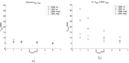
where the current drive efficiency η is a function of position. The broadening of the power profile applies also to the current density profile apart for the variation of η across the deposition profile, which is usually negligible for localized EC deposition. A general formulation of the power threshold to mitigate NTMs is discussed for example in [9], which is largely based on the analyses of the generalized Rutherford equation presented in [45, 46]. We may repeat the calculation assuming the beam driven current is broadened by factor of 1, 2 or 3. The resulting power is shown in figure 15. The conclusions of [9] still remain valid: with the broadened beams continuous wave injection (cw) demands more than the nominal power available in the EC UL (13.3 MW per row of mirrors, ≈20 MW in total [9]), while the modulated (mod) power is still managable. Although in this case the whole UL might need to be reserved for NTM suppression only.
Figure 15. Power required for complete  NTM suppression as a function of marginal island width for beam with nominal power deposition profile (a), broadened by a factor of 3. Similar figure with the broadening by a factor of two was published in [9]. Reproduced with permission from [9]. © 2015 EURATOM.
Download figure:
Standard image High-resolution image
5. Summary
To summarize, in this paper we have presented simulations of electron cyclotron wave propagation and absorption in ITER, retaining the effects of scattering due to edge density fluctuations. This is particularly important for the upper launcher of ITER because of NTM stabilization. The simulations were carried out using WKBeam code that was benchmarked against paraxial beam-tracing code TORBEAM and full-wave IPF-FDMC code. In particular, we showed that the Born approximation utilized in the WKBeam code is applicable in the parameter range of ITER. We analyzed the scattering operator which describes the effects of turbulence on the wave, showing that the radiative transport due to density fluctuation can be of diffusive or superdiffusive nature. Moreover, it was shown that nominal parameters for ASDEX Upgrade tokamak lie barely in the superdiffusive regime while ITER is deeply in the diffusive regime. Because of this, and because of the larger machine size, a larger beam broadening can be expected in ITER.
The input needed for the averaged scattering includes statistical averages over the turbulence, namely the fluctuation amplitude  , that was assumed to be a function of radial coordinate
  and the poloidal geometrical angle θ, and the perpendicular correlation length
  . Based on our present knowledge, and 'educated guesses' for the value of these quantities in the ITER 15 MA standard H-mode scenario, extensive scans have been performed in order to assess the sensitivities of the results to the relevant parameters. Thereafter, simulations were carried out to calculate the beam broadening defined as a increase of the FHWM of the absorption profile. Broadening by a factor of 1.7 to 5.1 was observed depending on the turbulence parameters. In the most likely regime of parameters a broadening by a factor of 2.5 to 3.5 is found. It was observed that the ballooning like poloidal dependence of the fluctuation amplitude decreases the broadening to levels found with half of the fluctuation amplitude without the ballooning, leading to roughly a decrease of broadening by a factor of 2. Parameter scans were shown for the most important turbulence parameters, i.e. the fluctuation level in the SOL and the correlation length. Last but not least, it was shown that, even with a factor of 3 broadening, NTM mitigation by ECCD in ITER is still plausible but modulation of EC power could become necessary to achieve NTM suppression within the available power.
6. Outlook
In this paper we concentrated on the most important ITER mission, i.e. the 15 MA standard H-mode and only in flat-top phase. The next steps include similar analysis in other time slices and scenarios. Moreover, ITER is equipped with equatorial launcher (EL) that is foreseen to be mostly used for plasma heating and control applications. Some recent work has been carried out to investigate whether this system could be used to drive current in the  surface to destabilize sawtooth [6, 47]. Therefore, the work will be extended to EL as well. Although in this paper we considered only beam broadening effects, the mode-to-mode scattering should not be forgotten. It is important both for NTM mitigation, as part of the power is not coupled to plasma, and to stray radiation studies. We expect mode-to-mode scattering to be important also for EL. Recent numerical development of WKBeam code aims to generalize the input magnetic field for full 3D geometry. This enables to study scattering phenomena in stellarators, in particular W7-X that is equipped with good diagnostics possible capable of measuring beam broadening. Furthermore, larger scale turbulent blobs and ELM structures might affect the propagation of EC waves. Future work to estimate this effect in terms of NTM mitigation is foreseen.
Acknowledgments
This work has been performed within Fusion for Energy Grant 615. The views expressed in this publication are the sole responsibility of the author and do not necessarily reflect the views of Fusion for Energy. We are thankful for the fruitful discussions with E. Wolfrum on electron density fluctuations profiles. The main author acknowledge discussion with W. Chang.
Footnotes
- 4
The flat top phase of Case#001 from [43] is used, which corresponds to the run with PPF file # 53 287/fkochl/jul2811/sequation 1/ppfsequation 17 416.