


Abstract
Besides strong geodesic acoustic mode (GAM) activity, turbulence in the I-mode confinement regime of ASDEX Upgrade exhibits two prominent features, the weakly coherent mode (WCM) and strongly intermittent solitary density perturbations. The nonlinear interaction between these structures is studied in detail by means of a conditional averaged wavelet-bicoherence analysis. The wavelet analysis reveals that these density perturbations are at the WCM frequency. The GAM is coupled to all frequency scales of the velocity fluctuations via a modulational instability. The WCM shows coupling to higher frequencies prior to the bursts, indicating a process resembling wave-steepening. A possible mechanism for the generation of such solitary density perturbations by a Korteweg–de Vries-like nonlinearity is discussed.
Export citation and abstract BibTeX RIS
This article was updated on 25 August 2021 to correct the copyright line.
1. Introduction
As large edge localized modes (ELMs) are a serious concern for reactors, and even for ITER, intrinsically ELM-free regimes with good confinement as the I-mode would be an attractive operating regime for a fusion reactor. The I-mode is an improved confinement regime of tokamak plasmas operating in the unfavorable ion  -drift direction, combining H-mode-like energy confinement with L-mode-like particle and impurity transport [1]. It was first described as the 'improved L-mode regime' on ASDEX Upgrade (AUG) [2], but the recent extensive studies in Alcator C-Mod [1, 3–7] have attracted attention as a possible operating scenario for ITER. An non-harmful disadvantage is provided by the high L–I threshold compared with the L–H threshold in a favorable ion
  -drift direction [8]. Furthermore, the I-mode in AUG [8] and DIII-D [9] often evolves slowly in an uncontrolled manner, until a transition to the H-mode with large ELMs occurs. This would negate all advantages of the I-mode. It has been observed in both AUG and Alcator C-Mod that the power threshold from L- to I-mode scales at most weakly with the magnetic field (
 in AUG [10] and
  in C-Mod [7]) whereas the L- to H-mode power threshold scales nearly linearly with B (
 [11]). This would enhance the operation window of the I-mode at higher magnetic fields compared with the small operating window faced in the majority of present-day tokamak experiments. At a magnetic field of 8 T no transitions to H-mode have been observed in Alcator C-Mod [7]. This indicates that at high magnetic fields the I-mode may be a promising operating regime for a fusion reactor. To qualify the I-mode as an operating scenario for ITER, threshold and accessibility studies [8] on a multi-machine basis [6] are needed.
In addition, studies of turbulence in I-mode may offer a better understanding of the physics of the interaction of energy and particle transport barriers in general. The mechanism which selectively reduces only one of the transport channels is not understood. In the present contribution the turbulence characteristics of I-mode plasmas in AUG have been studied in detail. Two prominent features, the weakly coherent mode (WCM) [12] and the appearance of strongly intermittent density bursts [13, 10] as well as their connection, are highlighted. Recent progress on confinement properties of I-mode plasmas in AUG will not be discussed in the present contribution but can be found in [8, 10]. The new results presented in this paper include a detailed (conditional averaged bispectral) wavelet analysis to account for the strong intermittent behavior of turbulence in the I-mode in AUG, a discussion of the kind of intermittency observed and a more detailed presentation of the suggestion for the generation of solitary waveforms by Korteweg–de Vries (KdV)-like nonlinearity, only briefly presented in [13], which is this time derived from the Braginskii equations.
2. Frequency spectra of fluctuations during I-mode
Experiments were carried out on the ASDEX Upgrade tokamak (AUG), which has major and minor horizontal radii of R0 = 1.65 m and a = 0.5 m, respectively. The toroidal magnetic field strength was B0 = −2.5 T and the plasma current was  MA. The presented discharges are in the upper-single null configuration, where the ion
  drift is directed away from the X-point providing the necessary high power threshold for H-mode access. The discharges discussed are representative of I-mode plasmas in AUG. Details on discharge parameters including background profiles can be found in [10, 12, 13].
The density fluctuations shown in figure 1(a) are measured by hopping reflectometry diagnostics [14]. At the transition to I-mode the broadband region splits up into two bands in frequency space, one at low frequencies (f < 30 kHz) and one at higher frequencies (80 < f < 150 kHz). The band at higher frequencies is called the WCM [3]. This is the general characteristic fluctuation feature of the I-mode [3]. It is located in the steep gradient region at the very edge of the plasma [12]. In AUG the WCM appears at frequencies around 100 kHz with a width of a few 10 kHz (figure 1)(a) [12]. The wavenumber of the WCM in AUG is at  cm−1 [12] similar to the Alcator C-Mod results [5]. In addition to the WCM a geodesic acoustic mode (GAM) appears (figure 1(b)). Any flow as the GAM advects small-scale (high frequency) structures which leads to a modulation of perturbations at higher frequency. Therefore the effect of a flow can be approximated by the low-frequency envelope of high-frequency perturbations. This has been estimated by the envelope of density fluctuations above 400 kHz measured by hopping reflectometry, as done in [15] and described in detail in [12, 16]. The GAM advects the WCM and leads to broadening through the Doppler effect [12]; this constitutes the energy transfer as seen in [5]. The basic instability of the WCM is still unknown, but recent simulations with BOUT++ indicate a simple drift-Alfénic instability [17].
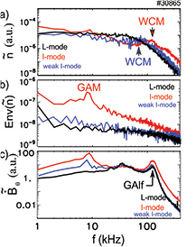
Figure 1. (a) Spectrum of density fluctuations from frequency hopping reflectometry, (b) its envelope deduced from density fluctuations and (c) poloidal magnetic field fluctuations in the L- (black) and I-mode (red). Also the spectra at the beginning of development of the I-mode (called the weak I-mode) are shown in blue.
Download figure:
Standard image High-resolution imageIn AUG, magnetic fluctuations close to the WCM are amplified during the I-mode (figure 1(c)). Using the measured background profiles the gyrokinetic eigenvalue solver LIGKA [18] is used to determine the kinetic continuum branches of toroidal symmetric modes. Two modes, the GAM (m = 0,  kHz) and a global Alfénic mode (m = 1,
  kHz) called the geodesic Alfénic mode (GAlf), are close to the experimentally observed frequencies. The GAlf is similar to the mode previously observed in TFTR [19]. The frequency of the magnetic fluctuations close to the WCM frequency coincides with the GAlf frequency [12]. Comparisons with Mirnov coils show the characteristic toroidal and poloidal mode numbers of the GAlf of zero and one, respectively [12]. However, these magnetic fluctuations are already present in the L-mode (figure 1(c)). As seen in the early weak I-mode (blue line in figure 1), where the pressure gradients just slightly steepen and the confinement just increases slightly at constant heating power [12], the frequency of the WCM (
 kHz, blue line in figure 1(a)) is smaller than the developed I-mode (
 kHz, red line in figure 1(a)). The magnetic fluctuations (GAlf) do not change (
 kHz, figure 1(c)) and WCM and GAlf do not coincide in frequency in the weak I-mode case. Therefore, it should be stressed WCM and GAlf are not the same mode.
3. Strongly intermittent density fluctuations
The edge turbulence in the L-mode is characterized by broadband fluctuations as measured by Doppler reflectometry (DR) in figure 2(a). While the background density turbulence level is reduced in the I-mode compared with the L-mode level, the I-mode in AUG exhibits strong intermittent density bursts (figure 2(b)) causing a heavy-tail probability distribution function (PDF) [10, 13]. The bursts exhibit a solitary waveform and last for about 2–10 μs [10, 13]. These bursts are not ELMs—the peeling–ballooning stability boundaries are far away from the experimental parameters in the I-mode as calculated with the MISHKA code [10]. Furthermore, no pronounced magnetic signature typical for type-I ELMs [20] is observed.
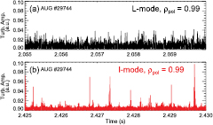
Figure 2. Comparison of turbulence amplitude behavior in (a) the L- and (b) the I-mode measured with Doppler reflectometry.
Download figure:
Standard image High-resolution imageTurbulence bursts also occur in the late I-phase [21]. However, the bursts in the I-phase appear more regular in time with a much longer duration. Also the bursts exhibit type-III ELM-like precursors in the late I-phase [22] which is usually not observed in the I-mode. The bursts in the I-mode show some similarities to inter-ELM fluctuations in the H-mode, as previously observed [23]. A detailed study on this similarity is left for future work.
Most importantly, the intermittent events show up in the divertor measured by absolute extended ultraviolet (AXUV) diode-based bolometry [24] several tens of microseconds later than observed with DR in the confined region at the minimum of the radial electric field [10]. The radiative response in the divertor is much longer in time than the bursts measured with the DR [10]. The divertor impact in combination with the strong density perturbation in the confined region suggests that these bursts are playing an important role in hampering the development of the density pedestal, although a proof by direct measurements of the particle transport is not possible as the bolometer measurement is a combination of density, temperature and impurity concentration.
Previous results show a strong correlation between density bursts and the WCM [13]. Complementary to the previous analysis [13], a wavelet-based approach is used here. For strongly intermittent time series containing short-lived events a wavelet analysis avoids averaging out temporally localized events compared with a Fourier-based analysis. The wavelet transform is given by
where the complex Morlet wavelet 
 is used here, where C is a real constant. Figure 3(a) shows the amplitude of density fluctuations in the I-mode measured by DR as a reference. (the square root of the squared I and Q signal is used). In figure 3(b) radiative fluctuations measured by AXUV bolometry at a line of sight measuring just outside the confined region in the upper divertor (DVC48) are shown. A general correlation is not that obvious. However, the strongest activity of the WCM at around t = 3.9384 s is accompanied by a clear radiative response in the upper divertor. Closer to the I–H transition the correlation between bursts and radiative fluctuations in the upper divertor is more evident, as shown in [10]. The wavelet transform of the density fluctuations measured by DR is shown in figure 3(c). The density bursts are perturbations at the WCM frequency at around 100 kHz. The wavelet analysis of the phase measured by conventional reflectometry also shows an intermittent activity of the WCM (figure 3(d)). Strong activity of global modes (such as the GAM or WCM) can lead to strongly localized turbulent activity. Due to turbulence localization the transport can become bursty [25]. The envelope of the phase fluctuations measured by conventional reflectometry, which is a measure of the velocity fluctuations, is investigated. The envelope is estimated from the high-pass filtered (above 400 kHz) phase fluctuations. Also, the envelope which can be seen as an approximation for the flow is fluctuating intermittently showing features at the GAM and WCM frequency (figure 3(e)).
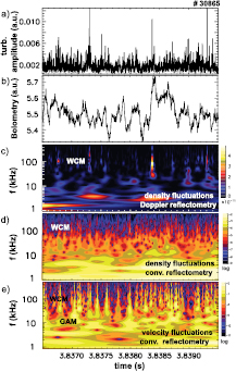
Figure 3. Turbulent amplitude of density fluctuations measured by Doppler reflectometry (a), radiative fluctuations at the upper divertor measured by AXUV bolometry (b), wavelet transform of these density fluctuations (c), of density fluctuations measured by conventional reflectometry (d) and of the envelope fluctuations as a proxy for velocity fluctuations measured by conventional reflectometry (e).
Download figure:
Standard image High-resolution imageAn intermittent behavior of the GAM is not unusual and has been reported from most devices [26–38]. Intermittent transport associated with the GAM has been studied theoretically near the critical gradient regime [39]. Where the GAMs emit turbulence energy in bursts, the energy of stationary zonal flows can accumulate gradually due to the undamped residues. This leads to a dynamic increase in turbulence quenching as well as to a nonlinear upshift of the critical gradient (i.e. the Dimits shift) [39]. This might be related to the observed spontaneous uncontrolled non-steady improvement of confinement of the I-mode which most often leads to a transition to H-mode [8].
4. On external and internal intermittency
The term intermittency describes two distinct aspects of turbulent flows [40]: these are not independent. The first one, so-called external intermittency, is associated with partly turbulent flows, with the strongly irregular and convoluted structure and random appearance of turbulent and non-turbulent fluid [40]. External intermittency is characterized by an on–off variation. This on–off variation induces strong deviation from Gaussian statistics [40]. This kind of intermittency is a key problem for renewable energy as solar generators only produce energy when the sun is shining or wind turbines only produce energy as the wind is blowing. Also intermittency in the context of critical phenomena, as in stock market dynamics or earthquakes for example, is related to this kind of intermittency and is not related to a particular scale as the on–off variation affects all scales. The second aspect is the so-called internal or small-scale intermittency, which is usually associated with the tendency to spatial and temporal localization of the fine- or small-scale structure of flows always in the turbulent state [40]. This kind of intermittency is related to dissipation at the smallest scales and possibly to a deviation from self-similarity in the large-wavenumber region.
The perpendicular wavenumber measured with the Doppler reflectometer has been scanned between  –10 cm−1. The deviation from Gaussian statistics increases with improving confinement [13, 10], as seen in figure 4, by the PDF of the density fluctuation amplitude. The density bursts are not only observed when small structures are probed but also at rather large scales. At large scales the development of the heavy tail in the PDF is even more pronounced. Therefore, intermittency in the I-mode seems not to be related to small-scale intermittency in particular, but first of all to external intermittency.
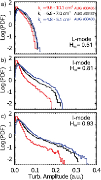
Figure 4. Probability distribution functions of density fluctuation amplitudes obtained at  for different sizes
  cm−1,
cm−1,  cm−1,
cm−1,  cm−1 shown at the same level of confinement in the L-mode (H98 = 0.51) (a) and I-mode (H98 = 0.81 (b) and H98 = 0.93 (c)). Heavy tails develop with improved confinement in the I-mode. Larger structures show more pronounced tails.
Download figure:
Standard image High-resolution imageExternal intermittency is a basic process of the transition from laminar to turbulent flow. At the transition from laminar to turbulent flow, laminar and turbulent regions coexist in the same flow. The Kármán vortex street is a well known example of this. This is consistent with the kind of intermittency observed by DR in the I-mode. The turbulence is strongly suppressed most of the time and the fluctuations are restricted to small periods in time. Interestingly there is a further similarity with a specific transition scenario to a turbulent state. The transition to drift-wave turbulence is found to follow the Ruelle–Takens scenario [41]. By increasing the control parameter the system passes through different regimes from periodic to quasi-periodic to mode locked to weakly turbulent. In the mode locked regime a quasi-coherent mode appears [42]. In this regime a large-scale flow structure is generated by the inverse energy cascade process and coupled to small-scale density fluctuations [43]. Through this coupling the density perturbations are phase locked and synchronized to the large-scale flow and appear as a quasi-coherent mode [43]. This appears to be similar to the WCM, where the density fluctuations are phase locked by the GAM [12]. From this point of view, the I-mode can be seen to be at the transition to turbulence. Also other high-confinement regimes exhibit quasi coherent modes and may be considered to be rather at the transition to turbulence than turbulent. For example in the usual H-mode quasi-coherent fluctuations also appear in the magnetics at high frequency [44, 45] and the turbulence level is small.
5. Nonlinear interaction between GAM, WCM and density bursts
To investigate the nonlinear coupling between GAM, WCM and the density bursts, the conditional averaged wavelet-bicoherence [46] is estimated. It is based on three existing techniques, wavelet analysis, bispectral analysis and conditional averaging. Bispectral analysis is used to investigate the nonlinear interaction between different frequencies. Nonlinear interactions take place in frequency and as well in wavenumber space and have to fulfill the three-wave-coupling condition in both frequency  and in wavenumber space
  . The Doppler reflectometer is sensitive only to one wavenumber and the three-wave coupling condition in wavenumber space cannot be fulfilled. For this reason a conventional reflectometer is used for the following bispectral analysis. The wavelet analysis is needed to investigate short-lived events like the density bursts in the I-mode and the conditional average provides the possibility to focus on these events. The density fluctuations (approximated by the circular phase signal as described above) are divided into overlapping subwindows of 1200 μs length and the wavelet transform is performed with a lowest frequency of 2.5 kHz. To avoid boundary effects, only the central part with a length of 400 μs is used for the following analysis. Via advection by the flow
  , the density
  is subject to a nonlinearity
  which can be studied by means of the cross-bicoherence of density fluctuations
  and the envelope
  representing the flow
Using the more direct measurement of the velocity provided by DR instead seems tempting, but density and velocity have to be measured at the same position. This cross-bicoherence gives the degree of phase locking between the three different modes  ,
,  and
and  and takes values between zero and one. Phase locking is a necessary condition for nonlinear coupling. As a trigger for the conditional average the density fluctuations have been bandpass filtered between 100 and 200 kHz to estimate the WCM activity. Fluctuating data of 250 ms (3.75–4.0 s) are conditionally averaged over 119 events (indicated by the brackets
  ) exceeding the standard deviation of the trigger signal by a factor of 2.5 at the rising edge of the bandpass-filtered (100–200 kHz) density perturbations. The corresponding significance level is about 0.01. The conditional averaged WCM density burst is shown in figure 5(a) (with the black line) together with the wavelet power spectrum of the density perturbations that have not been bandpass filtered but conditionally averaged with the same condition. An increase in the WCM amplitude is observed. Compared with the envelope fluctuations it is observed that the WCM fluctuations in the density (figure 5(a)) are accompanied by velocity fluctuations (figure 6(a)).

Figure 5. Conditional averaged density burst (black, a), conditional averaged wavelet power spectrum of density fluctuations (a), the conditional averaged cross-bicoherence  at
at  μs (b),
  μs (c) and
  μs (d) with respect to the conditional averaged WCM density burst.
Download figure:
Standard image High-resolution image
Figure 6. Conditional averaged WCM density burst (black, as in figure 5(a)), conditional average of the wavelet power spectrum of the envelope fluctuations (a), the conditional averaged auto-bicoherence  at
at  μs (b),
  μs (c) and
  μs (d) with respect to the conditional averaged WCM density burst.
Download figure:
Standard image High-resolution image
In the following, the general coupling features are described. In I-mode a pronounced coupling of the center of gravity proportional to velocity fluctuations at low frequency of the GAM-like mode (∼10 kHz) with the WCM (70–140 kHz) is found (see (A) in figures 5(b)–(d)), as reported previously [12]. The velocity fluctuations of the WCM ( ) are coupled to fluctuations near the WCM frequency (
 ) and the second harmonics of the WCM band (f1 = 140–280 kHz) (see (B) in figures 5(b) and (c)). The coupling between the GAM-like mode and WCM can be also observed in the auto-bicoherence of the envelope fluctuations
This resembles the effects of the nonlinearity  in the polarization equation, responsible for the inverse energy cascade and structure formation including the Reynolds stress. In general, the GAM frequency is coupled to all other frequencies, indicating the modulation instability [47, 48] which is equivalent to the Reynolds stress drive of the GAM. Here, the GAM is primarily coupled to the WCM (see (A) in figures 6(b)–(d)) and once higher frequencies are excited these are also coupled to the GAM, as indicated by the extension of the lines in the center.
Next, the time dependence of the nonlinear coupling process is described. At  μs the velocity fluctuations of the WCM are coupled to higher frequencies f1 > 140 kHz in the density (see (B) in figure 5(b)). This coupling increases with time. At
  μs velocity fluctuations at the WCM frequency
  are coupled to themselves, generating higher harmonics (see (C) in figure 6(b)). The induced high-frequency velocity fluctuations can now modulate the density, leading to perturbations at higher frequencies in the density (see (D) in figure 5(c)) as well in the velocity (see (E) in figure 6(c)). As in a self-steepening process, higher and higher frequencies are becoming involved in the generation of the burst.
One of the main reasons for small-scale intermittency is thought to be the direct interaction (or non-local coupling) of large and small scales [40, 49]. Small-scale intermittency spends a very short time at very small scales. The power and amplitudes at high wavenumbers (small scales) and short times (high frequencies) are small. To be intermittent, the power, which is at large scales, has to be transmitted to small scales in a very short time. Non-local coupling in wavenumber space provides such a possibility. Even though intermittency in the I-mode is a type of external intermittency, the energy has to be transmitted from low to high frequencies also in this case. Non-local coupling between large and small scales is observed here by the coupling of the GAM-like mode at large scales with the WCM at smaller scales and even smaller scales of the bursts, and might be the reason for the intermittency. It should be noted that only the possibility of energy transfer and not the net energy transfer is measured by the bicoherence. If the basic instability of the WCM grows, it is suppressed by the Reynolds stress (see (A) in figures 6(b)–(d)). This suppression occurs due to the transfer of kinetic energy from the WCM and all other modes to the GAM. The energy transfer is proportional to the flow shear [50], which is higher for higher confinement.
6. Generation of solitary-like structures
The density bursts exhibit a solitary waveform. Solitons are a result of a competition between self-steepening by a nonlinearity and dispersion, as described for example in 1D by the KdV equation. The nonlinearities appearing in the KdV and Burgers equations are known to be responsible for intermittency in 1D systems [51]. Self-steepening results in the generation of higher harmonics. This is not possible for the standard nonlinearity in a magnetized plasma given by the advection by the  drift
drift  , with magnetic field
  in the
  direction and strength B and electrostatic potential
  . It can be written as
  with electron temperature Te, elementary charge e and
  . In wavenumber space
  this is proportional to
  . Therefore higher harmonics
  with constant scalar c cannot be generated directly. The observation of the generation of higher harmonics in the bispectrum ((B) in figure 5) is not as trivial as it seems.
Here, one possibility for the generation of such solitary-like structures is shown. The starting point is the advective part of the electron temperature of the Braginskii equation [52]
In the next step, temperature and density are divided by typical values, n0 and Te0, respectively. The normalized density and temperature are decomposed in background and fluctuating quantities  and
and  . Making use of the Poisson bracket
  , with x the radial and y the binormal coordinate, the advective part can be written as
In drift-wave ordering, the gradients of the fluctuations are in the order of the gradients of the background values, therefore the first term is the highest in drift-wave ordering and the last two terms would be neglected. As a product of three fluctuating quantities the third term is negligibly small. However, the second term can be written as
and in the case of these strong density bursts in the I-mode, the density fluctuation level as well as the background temperature gradient are considered to be high. On the other hand, the first term in competition is proportional to the temperature fluctuation level, which is considered to be low. This has been observed to be the case in Alcator C-Mod [53]. A confirmation in AUG is still pending. The transition of the dominant turbulence regime from drift-wave dominated to resistive ballooning dominated is expected to occur at  [54], where the local normalized collisionality is given by
  and
and  with electron and ion masses me and mi, respectively, safety factor q, collisionality
  and ion sound speed
  . For
. For  m−3,
m−3,  eV, q = 5 and
  cm at
cm at  we get
  and
and  , hence
  . It seems reasonable at these low collisionalities at high temperatures to assume adiabatic electrons with
  . In this case the nonlinearity has the form ∼
 of a KdV nonlinearity explicitly proportional to the radial temperature gradient. Therefore, drift-wave turbulence with intrinsically low transport can generate solitary-like temperature perturbations. How are those transmitted to the density? The adiabatic coupling including temperature perturbations is given by
  [52]. The temperature fluctuations can be approximated by
  . For low temperature fluctuations
  is still valid. Therefore there is no contradiction with the argument above. Defining a small phase difference δ between potential and density fluctuations with
  , it follows
  . Density fluctuations can be induced by the temperature fluctuations as
  . If the phase difference δ is small the bursts appear larger in the density than in the temperature. The temperature fluctuations also lead to particle transport
  . With the
  response this can be written as
  . The associated heat transport is
  which is small as
  is small and in the opposite direction to the particle transport.
One possible scenario for the generation of solitary-like density perturbations regulating the particle transport is the following: a close to adiabatic coupling between potential and density can induce a solitary-like perturbation in the electron temperature if the density fluctuation level and the electron temperature gradient are high and the electron temperature fluctuation level is low. This temperature perturbation can be proportional to the phase shift between potential and density and an increase in the temperature fluctuation level can lead to an increase in particle transport accompanied by a soliton-like waveform in the density induced by the adiabatic coupling. By means of line ratio spectroscopy on helium [55] or correlation electron cyclotron emission [56] it may be possible in the near future in AUG to measure density and temperature fluctuations at the same point in space and time and hence their cross-phase allowing a quantitative examination of the presented scenario.
7. Summary
Recent studies of I-mode turbulence in AUG have shown two prominent features, the weakly coherent mode [12] and strongly intermittent density bursts [13]. The divertor impact in combination with the strong density perturbation in the confined region suggests that these bursts are playing an important role in hampering the development of the density pedestal [10]. As indicated in [10] and shown by the wavelet analysis here (figure 3) both features are strongly coupled. In AUG the short-lived (2–10 μs) intermittent density fluctuations measured by DR (at  –13 cm−1) appear at the WCM frequency. The WCM measured by conventional reflectometry (at smaller
  –2 cm−1) also shows an intermittent behavior. A strong activity of global modes (the GAM in the I-mode case) leads to strongly localized turbulent activity. Heavy tails in the PDF of the density fluctuation amplitudes are more pronounced at larger scales. Together with the on–off variation of the fluctuations, intermittency in the I-mode seems to be an external intermittency at the transition to turbulence in a phase-locked regime. Due to high turbulent amplitudes, nonlinear processes are becoming more important and the transport can become bursty [25]. The WCM in density measured by conventional reflectometry is accompanied by fluctuations in the envelope of high-frequency fluctuations at the WCM frequency. The envelope fluctuations can be interpreted as flow perturbations at the WCM frequency. These fluctuations also modulate density and velocity fluctuations at even higher frequencies. The nonlinear behavior during strong WCM activity shows an increase in high-frequency activity similar to a wave-steepening process. A KdV-like nonlinearity could be responsible for the intermittent behavior and the solitary waveforms, as observed in the experiment [13]. The explicit temperature gradient dependence of this nonlinearity may explain why the bursts are that pronounced in the I-mode [13]. This nonlinearity also provides the possibility to selectively reduce only one of the transport channels. However, this possibility awaits verification until combined fast temperature and density measurements are available.
Acknowledgments
This work has been carried out within the framework of the EUROfusion Consortium and has received funding from the Euratom research and training programme 2014–2018 under grant agreement no. 633053. The views and opinions expressed herein do not necessarily reflect those of the European Commission.